本文最后更新于 2025-03-09T19:44:28+08:00
百分比近似软阴影
若要判断当前着色点是否处于阴影之中,我们需要知到该点与光源之间的遮挡关系。一种常见的做法是 Shadow Mapping,假设从光源看向场景,就像做深度测试一样,保存一张从光源处获得的 DepthBuffer,然后比较着色点与光源之间的距离与 DepthBuffer 中对应点的深度,前者更大则代表场景中有另一物体比当前着色点更接近光源,即该着色点被遮挡。
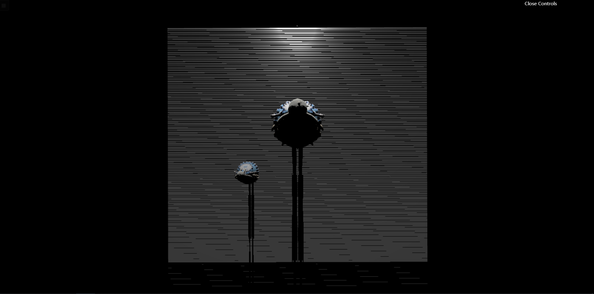
Two Pass Shadow Map 硬阴影
1
2
3
4
5
6
7
8
9
10
11
12
13
14
15
16
17
18
19
20
21
22
float useShadowMap(sampler2D shadowMap, vec4 coord) {vec4 closestDepthVec = texture2D (shadowMap, coord.xy);float closestDepth = unpack(closestDepthVec);return coord.z < closestDepth + 0.011 ? 1.0 : 0.0 ;void main(void ) {vec3 shadowCoord = vPositionFromLight.xyz / vPositionFromLight.w;0.5 + 0.5 ;vec3 phongColor = blinnPhong();float visibility = 1.0 ;vec4 (shadowCoord, 1.0 ));gl_FragColor = vec4 (phongColor * visibility, 1.0 );
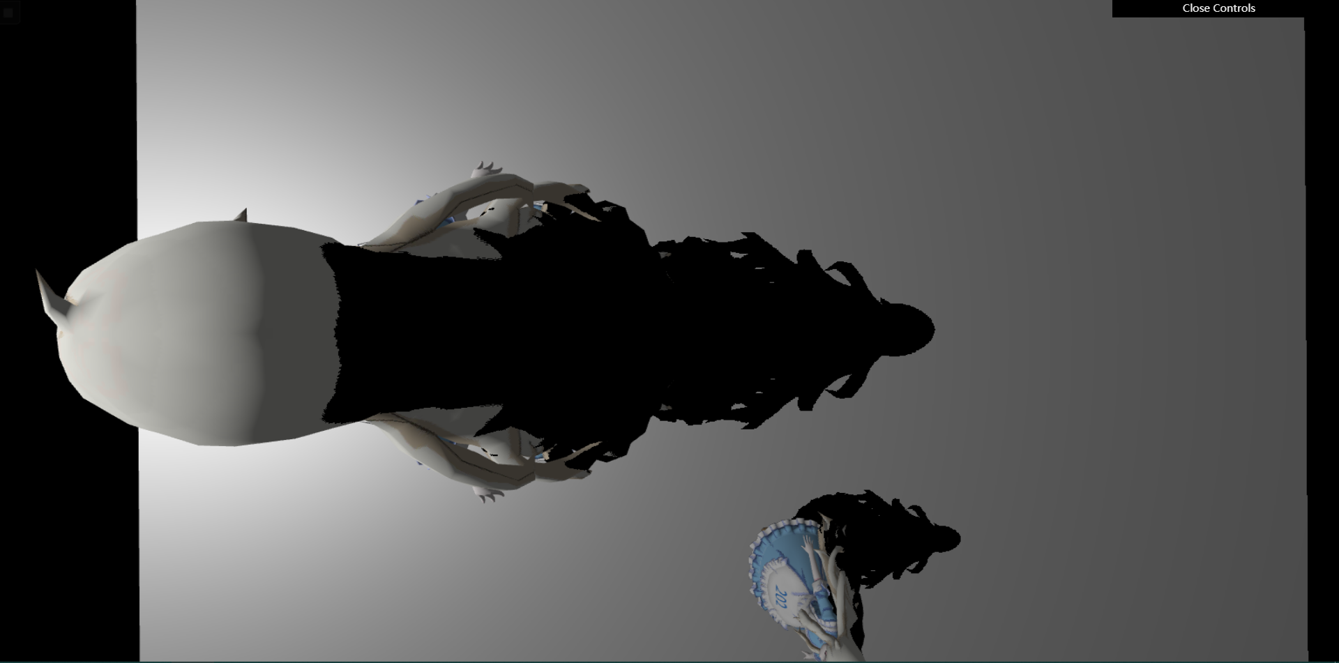
coord.z < closestDepth ? 1.0 : 0.0 的问题
这个问题源自于 Shadow Map 对场景走样/失真的理解。光源对场景的离散化认为 Shadow Map 内每一个纹素对应的表面属于同一个深度,此时对于侧对光源的表面,单个纹素内无法表示表面深度剧烈的变化,Shadow Map 便会将平面理解为一个…搓衣板。解决方法 :为判断条件添加一个容忍度。return coord.z < (closestDepth + 0.01) ? 1.0 : 0.0;新的问题 :当这个容忍度较大时阴影的根部会与模型发生分离,这个问题是目前难以解决的。
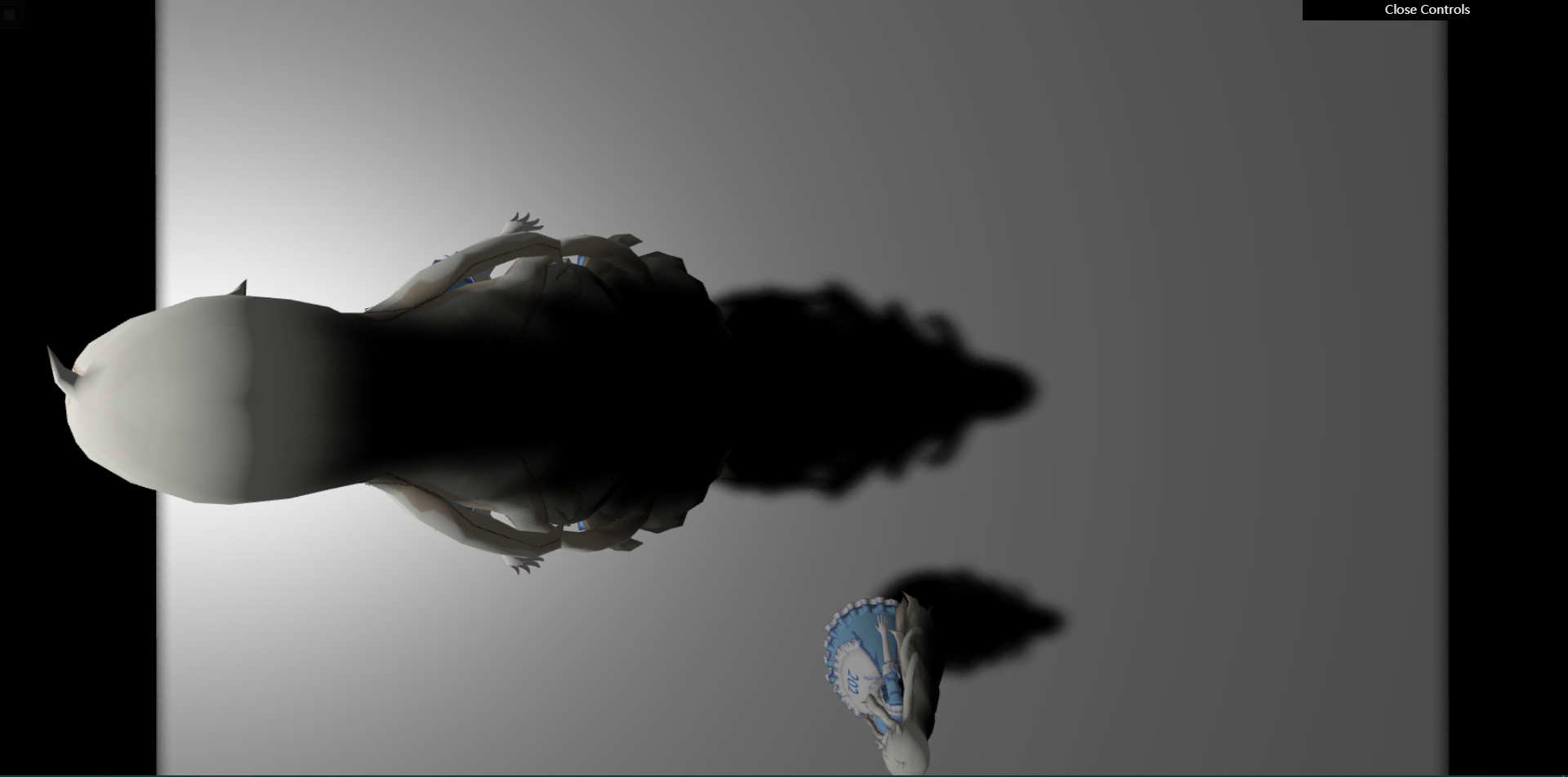
Percentage Closer Filter
不再仅仅查询 DepthBuffer 中对应点的深度,而是计算一定范围内深度大于着色点深度的比例,认为深度小于着色点深度的物体会遮挡着色点。
1
2
3
4
5
6
7
8
9
10
11
12
13
14
15
float PCF(sampler2D shadowMap, vec4 coord) {int unShadowCount = 0 ;for (int i = 0 ; i < NUM_SAMPLES; i ++) {vec2 sampleCoord = poissonDisk[i] * FILTER_DIAMETER + coord.xy;vec4 closestDepthVec = texture2D (shadowMap, sampleCoord); float closestDepth = unpack(closestDepthVec);if (coord.z < closestDepth + 0.011 ) {1 ;return float (unShadowCount) / float (NUM_SAMPLES);
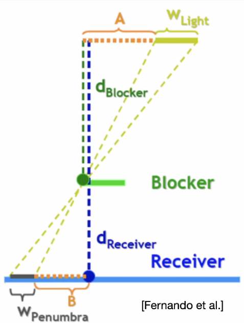
Percentage Closer Soft Shadow
PCF 的问题 :整体的阴影都会获得一个模糊,而现实情况是阴影的根部往往是最“扎实”的,远端的阴影才会渐渐变得模糊。解决方法 :已知阴影模糊的程度取决于 Filter 的大小,如果能让 Filter 的大小随阴影着色点与遮挡物的距离增加而增加,便能实现较为真实的软阴影。
avgblocker depth
calculate penumbra size
filtering (PCF)
avgblocker depth
在一定范围内查找能够遮挡着色点的物体的深度平均值。
1
2
3
4
5
6
7
8
9
10
11
12
13
14
15
16
17
float findBlocker(sampler2D shadowMap, vec2 uv, float zReceiver) {int shadowCount = 0 ;float blockDepthSum = 0.0 ;for (int i = 0 ; i < NUM_SAMPLES; i++) {vec2 sampleCoord = poissonDisk[i] * FILTER_DIAMETER + uv;vec4 closestDepthVec = texture2D (shadowMap, sampleCoord);float closestDepth = unpack(closestDepthVec);if (zReceiver > closestDepth + 0.011 ) {1 ;return blockDepthSum / float (shadowCount);
calculate penumbra size
根据第一步得到的遮挡物深度计算阴影的模糊程度。
W P e n u m b r a = ( d R e c e i v e r − d B l o c k e r ) ∗ W L i g h t / d B l o c k e r W_{Penumbra}=(d_{Receiver}-d_{Blocker})*W_{Light}/d_{Blocker} W P e n u mb r a = ( d R ece i v er − d Bl oc k er ) ∗ W L i g h t / d Bl oc k er
1
2
3
4
5
6
7
8
9
10
11
12
13
14
15
16
17
18
19
20
21
22
23
24
float PCSS(sampler2D shadowMap, vec4 coord) {float zReceiver = coord.z;float zBlocker = findBlocker(shadowMap, coord.xy, zReceiver);if (zBlocker <= EPS) return 1.0 ;if (zBlocker >= 1.0 ) return 0.0 ;float wPenumbra = W_LIGHT * (zReceiver - zBlocker) / zBlocker;int unShadowCount = 0 ;for (int i = 0 ; i < NUM_SAMPLES; i ++) {vec2 sampleCoord = poissonDisk[i] * FILTER_DIAMETER * wPenumbra + coord.xy;vec4 closestDepthVec = texture2D (shadowMap, sampleCoord); float closestDepth = unpack(closestDepthVec);if (zReceiver < closestDepth + 0.011 ) {1 ;return float (unShadowCount) / float (NUM_SAMPLES);
结果
预计算辐射传递
如何计算环境光照可以近似为一个 ManyLight 的问题,在这种情况下,如果想要得知某一着色点获得的光照,需要对该点的上半球进行采样,这会是一个非常大的性能开销。使用 PRT 的做法可以使用预计算的数据,在实时的条件下实现环境光照。未实现:球谐函数的快速旋转。
前置知识
Product Integral
∫ Ω f ( x ) g ( x ) d x \int _\Omega f(x)g(x)dx ∫ Ω f ( x ) g ( x ) d x
基函数
f ( x ) = ∑ c i ⋅ B i ( x ) f(x)=\sum c_i\cdot B_i(x) f ( x ) = ∑ c i ⋅ B i ( x )
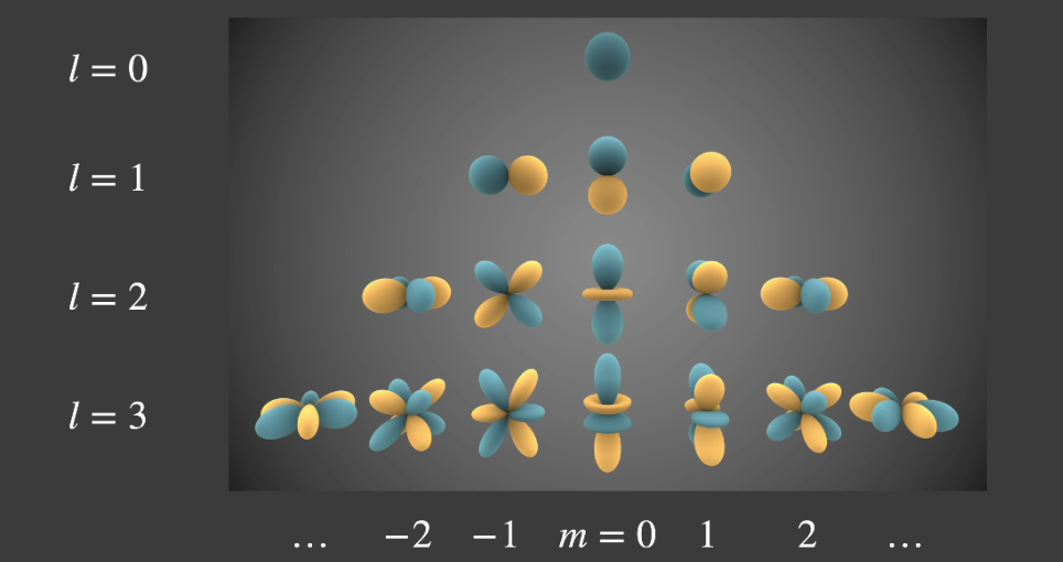
球谐函数
定义 :1 sin θ ∂ ∂ θ ( sin θ ∂ Y ∂ θ ) + 1 sin 2 θ ∂ 2 Y ∂ φ 2 + l ( l + 1 ) Y = 0 \frac{1}{\sin \theta}\frac{\partial}{\partial \theta}(\sin \theta \frac{\partial Y}{\partial \theta})+\frac{1}{\sin ^2\theta}\frac{\partial ^2Y}{\partial \varphi ^2}+l(l+1)Y=0 s i n θ 1 ∂ θ ∂ ( sin θ ∂ θ ∂ Y ) + s i n 2 θ 1 ∂ φ 2 ∂ 2 Y + l ( l + 1 ) Y = 0
c i = ∫ Ω f ( ω ) B i ( ω ) d x c_i=\int _\Omega f(\omega)B_i(\omega){\rm d}x c i = ∫ Ω f ( ω ) B i ( ω ) d x 正交性,任意两分量相乘结果为零。
旋转不变性,旋转的结果可由同阶基函数的线性组合得到。
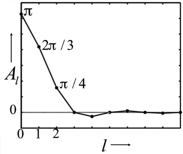
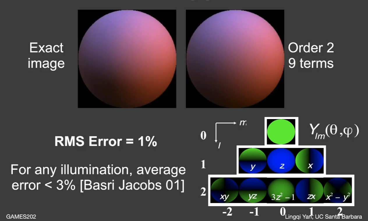
只用三阶的球谐函数便可以很好地恢复出渲染方程中的 BRDF 项。
所以对于 Diffuse 材质,同样用三阶的球谐函数表示 Lighting 项,误差不会超过 %3。
Precomputed Radiance Transfer
先写出实时渲染中渲染方程的形式:
L ( o ) = ∫ Ω L ( i ) V ( i ) ρ ( i , o ) m a x ( 0 , n ⋅ i ) d i L(o)=\int _\Omega L(i)V(i)\rho (i, o)max(0, n\cdot i)di L ( o ) = ∫ Ω L ( i ) V ( i ) ρ ( i , o ) ma x ( 0 , n ⋅ i ) d i
积分中 L(i) 当作 Lighting 项,其余为 LightTransport 项。假设场景中的物体不变(即每个点的 LightTransport 就像该点的一个性质一样不变),光源可以旋转。
Diffuse 的情况
BRDF 项为一个常值,可以直接提到积分外。
L ( o ) = ρ ∫ Ω L ( i ) V ( i ) m a x ( 0 , n ⋅ i ) d i L(o)=\rho \int _\Omega L(i)V(i)max(0, n\cdot i)di L ( o ) = ρ ∫ Ω L ( i ) V ( i ) ma x ( 0 , n ⋅ i ) d i
由 L ( i ) ≈ ∑ l i B i ( i ) L(i)\approx \sum l_iB_i(i) L ( i ) ≈ ∑ l i B i ( i )
L ( o ) ≈ ρ ∑ l i ∫ Ω B i ( i ) V ( i ) m a x ( 0 , n ⋅ i ) d i L(o)\approx \rho \sum l_i\int _\Omega B_i(i)V(i)max(0, n\cdot i)di L ( o ) ≈ ρ ∑ l i ∫ Ω B i ( i ) V ( i ) ma x ( 0 , n ⋅ i ) d i
由 c i = ∫ Ω f ( ω ) B i ( ω ) d x c_i=\int _\Omega f(\omega)B_i(\omega){\rm d}x c i = ∫ Ω f ( ω ) B i ( ω ) d x
L ( o ) ≈ ρ ∑ l i T i L(o)\approx \rho \sum l_iT_i L ( o ) ≈ ρ ∑ l i T i
Precompute 部分
c i = ∫ Ω f ( ω ) B i ( ω ) d x c_i=\int _\Omega f(\omega)B_i(\omega){\rm d}x c i = ∫ Ω f ( ω ) B i ( ω ) d x
使用黎曼积分的方式计算。
c i = ∑ i f ( ω ) B i ( ω ) Δ ω c_i=\sum _if(\omega)B_i(\omega)\Delta \omega c i = ∑ i f ( ω ) B i ( ω ) Δ ω
std::vector<Eigen::Array3f> PrecomputeCubemapSH(const std::vector<std::unique_ptr<float[]>> &images, const int &width, const int &height, const int &channel)
1
2
3
4
5
6
7
8
9
10
11
12
13
14
15
16
17
18
19
20
21
22
23
24
25
26
27
for (int i = 0 ; i < 6 ; i++) {for (int y = 0 ; y < height; y++) {for (int x = 0 ; x < width; x++) {int index = (y * width + x) * channel;Eigen::Array3f Le ( images[i][index], images[i][index + 1 ], images[i][index + 2 ]) float w = CalcArea (x, y, width, height); for (int l = 0 ; l <= SHOrder; l++) {for (int m = -l; m <= l; m++) {int k = sh::GetIndex (l, m);double basisFunc =EvalSH (l, m, dir.cast <double >().normalized ());
void preprocess(const Scene *scene)
1
2
3
4
5
6
7
8
9
10
11
12
13
14
15
16
17
18
19
20
21
22
23
24
25
26
27
28
29
for (int i = 0 ; i < mesh->getVertexCount (); i++) const Point3f &v = mesh->getVertexPositions ().col (i);const Normal3f &n = mesh->getVertexNormals ().col (i);auto shFunc = [&](double phi, double theta) -> double {ToVector (phi, theta);const auto wi = Vector3f (d.x (), d.y (), d.z ());double H = wi.dot (n);if (m_Type == Type::Unshadowed) {if (H > 0 ) {return H;return 0 ;else {ray (v, wi.normalized ());if (H > 0 && !scene->rayIntersect (ray)) {return H;return 0 ;auto shCoeff = sh::ProjectFunction (SHOrder, shFunc, m_SampleCount);for (int j = 0 ; j < shCoeff->size (); j++) {col (i).coeffRef (j) = (*shCoeff)[j];
结果保存在 light.txt 与 transport.txt 中。
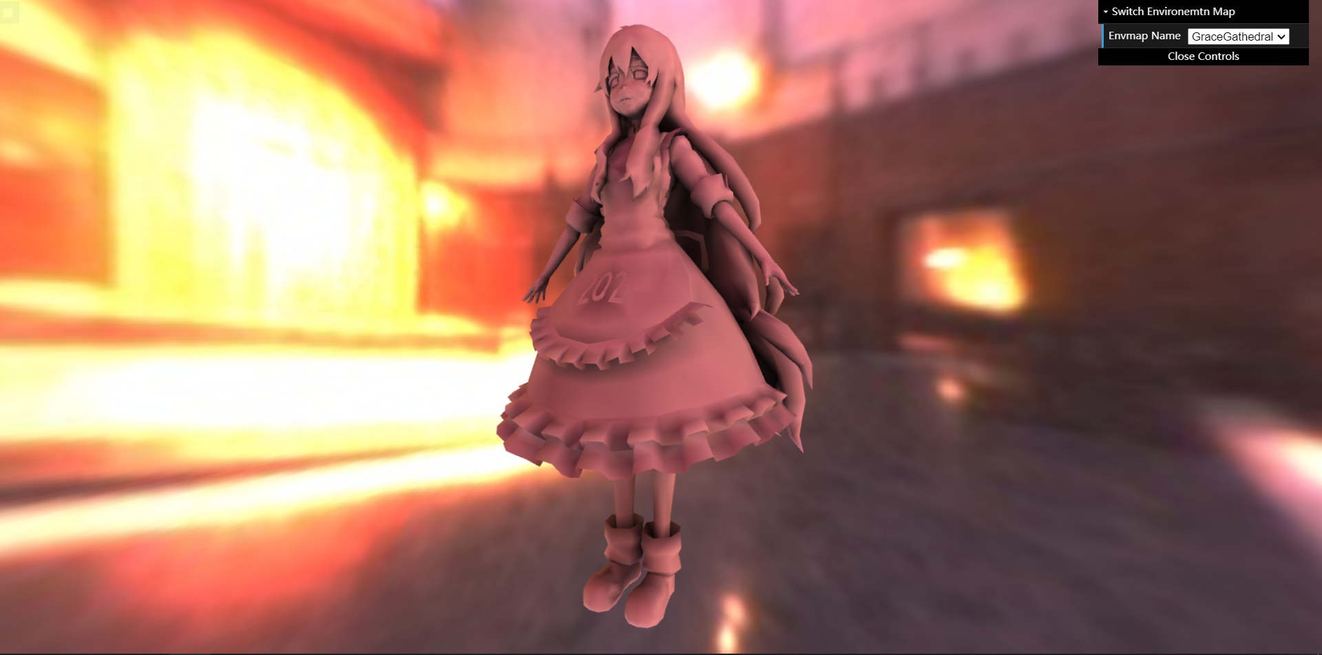
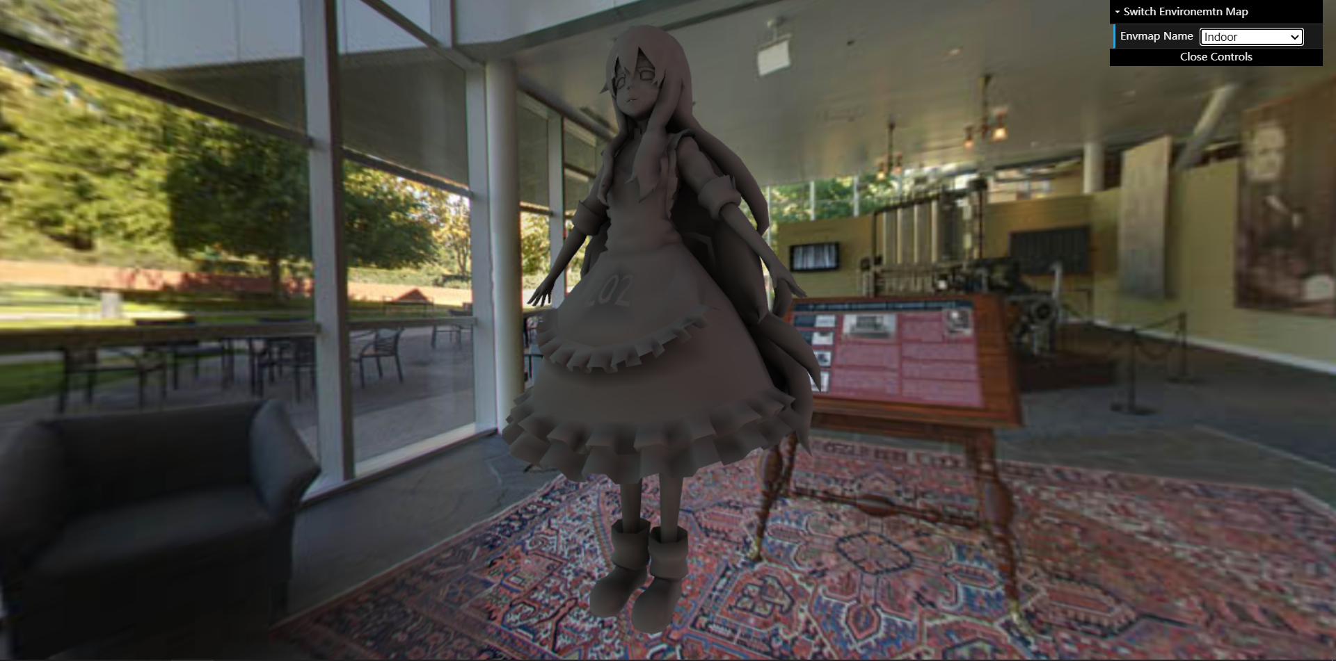
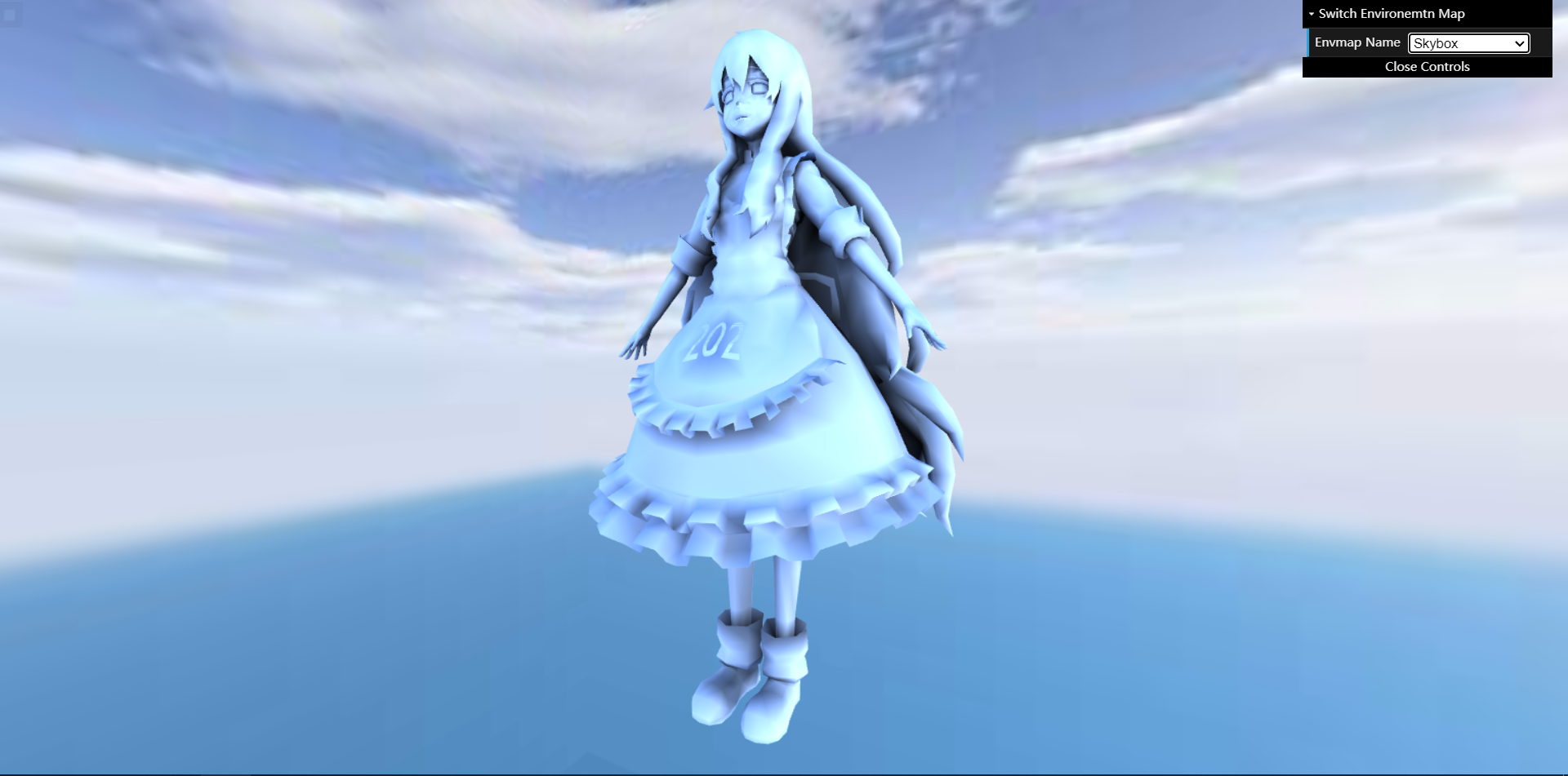
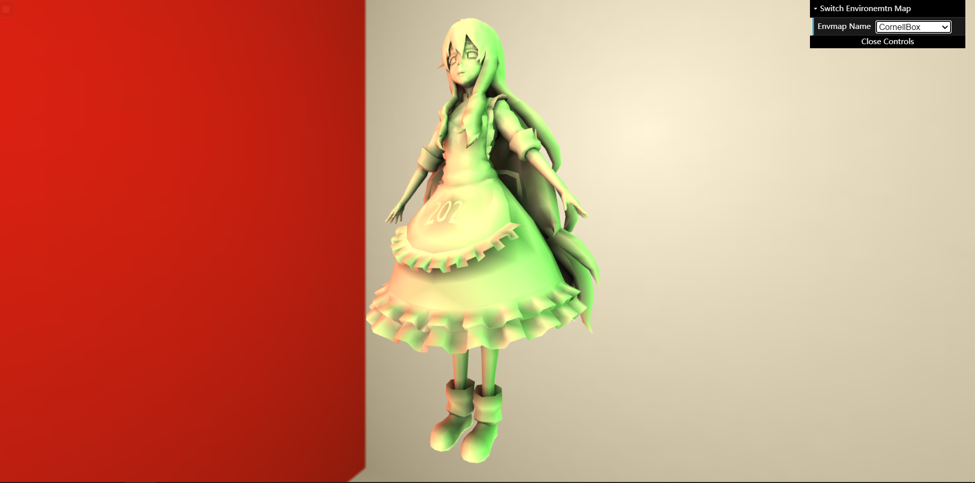
Real Time 部分
材质
1
2
3
4
5
6
7
8
9
10
11
12
13
14
15
16
17
18
19
20
class DiffuseMaterial extends Material {constructor (vertexShader, fragmentShader ) {let precomputeL_mat = getMat3ValueFromRGB (precomputeL[guiParams.envmapId ]);super ({'aPrecomputeLR' : { type : 'matrix3fv' , value : precomputeL_mat[0 ]},'aPrecomputeLG' : { type : 'matrix3fv' , value : precomputeL_mat[1 ]},'aPrecomputeLB' : { type : 'matrix3fv' , value : precomputeL_mat[2 ]}'aPrecomputeLT' ], vertexShader, fragmentShader, null );this .mapid = guiParams.envmapId ;async function buildDiffuseMaterial (vertexPath, fragmentPath ) {let vertexShader = await getShaderString (vertexPath);let fragmentShader = await getShaderString (fragmentPath);return new DiffuseMaterial (vertexShader, fragmentShader);
VertexShader
1
2
3
4
5
6
7
8
9
10
11
12
13
14
15
16
17
18
19
20
21
22
23
24
25
26
27
28
29
30
31
32
33
34
35
36
uniform mat3 aPrecomputeLR;uniform mat3 aPrecomputeLG;uniform mat3 aPrecomputeLB;attribute mat3 aPrecomputeLT;attribute vec3 aVertexPosition;attribute vec3 aNormalPosition;attribute vec2 aTextureCoord;uniform mat4 uModelMatrix;uniform mat4 uViewMatrix;uniform mat4 uProjectionMatrix;varying highp vec2 vTextureCoord;varying highp vec3 vFragPos;varying highp vec3 vNormal;varying highp vec3 vColor;const float kd = 2.0 ;const float pi = 3.14159 ;void main(void ) {vec4 (aVertexPosition, 1.0 )).xyz;vec4 (aNormalPosition, 0.0 )).xyz;vec3 iden = vec3 (1.0 , 1.0 , 1.0 );vec3 (dot (matrixCompMult (aPrecomputeLR, aPrecomputeLT) * iden, iden),dot (matrixCompMult (aPrecomputeLG, aPrecomputeLT) * iden, iden),dot (matrixCompMult (aPrecomputeLB, aPrecomputeLT) * iden, iden)gl_Position =vec4 (aVertexPosition, 1.0 );
FragmentShader
1
2
3
4
5
6
7
8
9
10
11
12
13
14
15
16
17
#ifdef GL_ES precision mediump float ;#endif uniform sampler2D uSampler;varying highp vec2 vTextureCoord;varying highp vec3 vFragPos;varying highp vec3 vNormal;varying highp vec3 vColor;void main(void ) {vec3 color = texture2D (uSampler, vTextureCoord).rgb;pow (color, vec3 (2.2 ));gl_FragColor = vec4 (vColor, 1.0 );
结果
屏幕空间反射
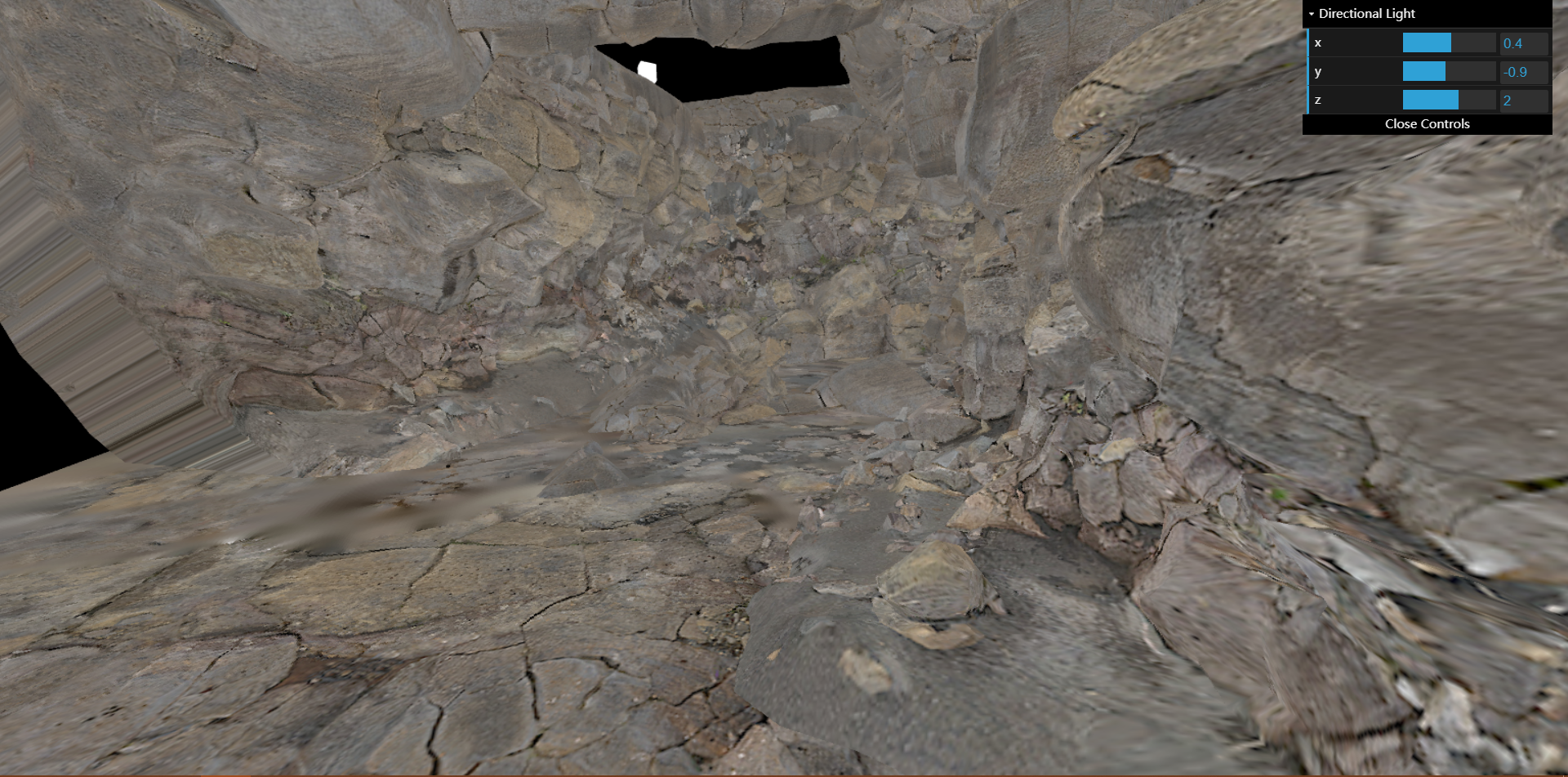
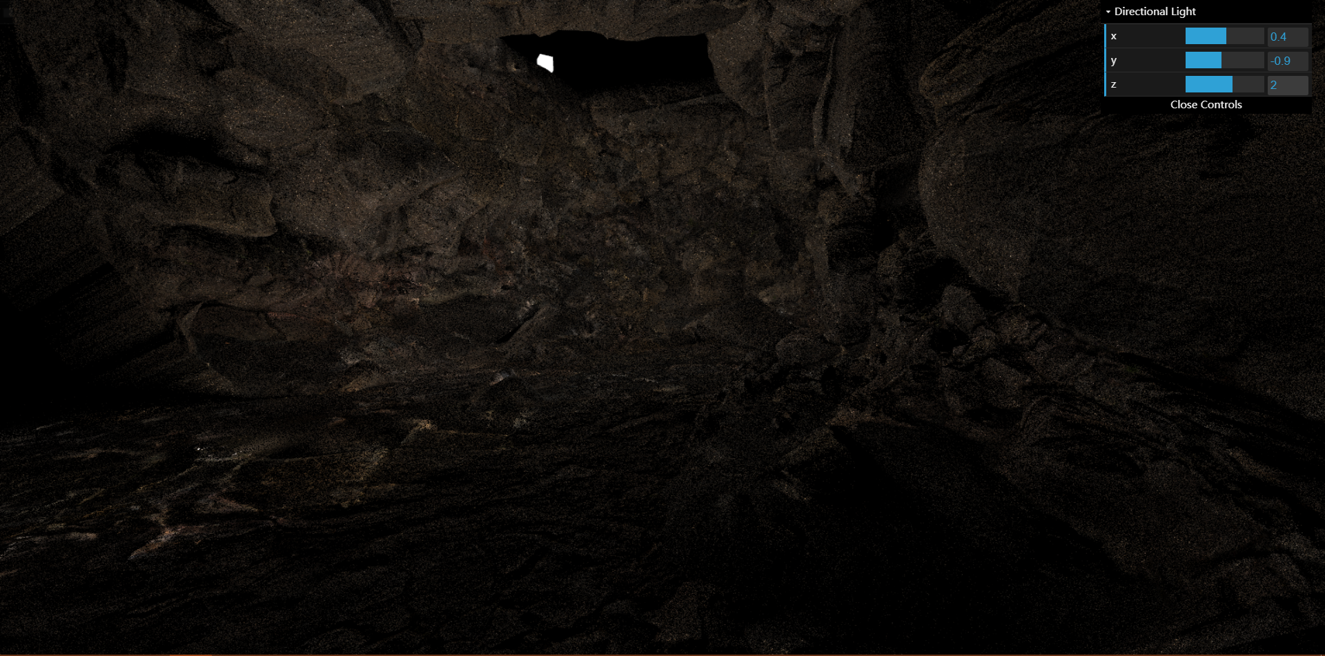
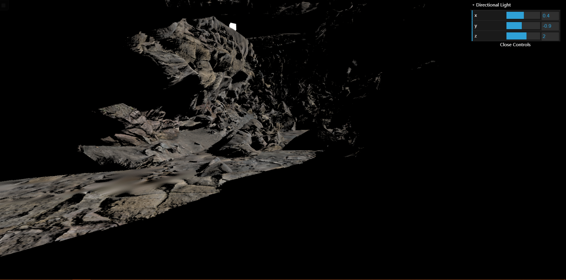
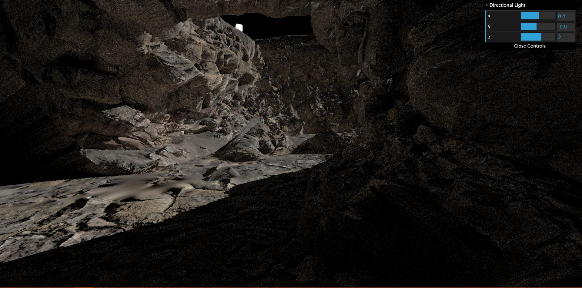
离线渲染的条件下,光线追踪可以处理光线在空间内的多次弹射,带来高质量的间接光照结果,那么如何在实时的条件下得到令人满意的全局光照效果呢。其中的一种做法是在做 RayTracing 时使用 DepthBuffer 判断射线与平面的相交问题,认为能被 DepthBuffer 看见得世界坐标是“位于物体外部”的坐标,看不见则在物体内部,那么一条步进的 Ray 从可见转为不可见时的位置便是某一表面所在的坐标,这样相交的计算就转变为二维空间下的步进与查表。
Shader
Diffuse
EvalDiffuse(wi, wo, uv) 的返回值为 BSDF 的值。参数 wi 和 wo 为世界坐标系中的值,分别代表入射方向和出射方向,这两个方向的起点都是着色点,uv 为着色点在屏幕空间中的坐标。
1
2
3
4
5
6
7
vec3 EvalDiffuse(vec3 wi, vec3 wo, vec2 uv) {vec3 Ld = GetGBufferDiffuse(uv);vec3 n = GetGBufferNormalWorld(uv);float nDotL = max (0.0 , dot (n, wi));return Ld * nDotL * INV_PI;
DirectionalLight
EvalDirectionalLight(uv) 的返回值为,着色点位于 uv 处得到的光源的辐射度,并且需要考虑遮挡关系,可以使用 GetGBufferuShadow(uv) 函数得到。
1
2
3
4
5
6
7
8
vec3 EvalDirectionalLight(vec2 uv) {vec3 woeldPos = GetGBufferPosWorld(uv);vec3 wi = normalize (uLightDir);vec3 wo = normalize (uCameraPos - woeldPos);vec3 bsdf = EvalDiffuse(wi, wo, uv);return uLightRadiance * bsdf * GetGBufferuShadow(uv);
RayMarch
RayMarch(vec3 ori, vec3 dir, vec3 hitPos) 的返回值为是否相交,相交时将参数 hitPos 设置为交点。参数 ori 和 dir 为世界坐标系,分别代表光线的起点和方向。
1
2
3
4
5
6
7
8
9
10
11
12
13
14
15
16
17
18
19
20
21
22
23
24
25
26
27
28
29
30
31
32
33
34
35
36
37
38
#define EPS 1e-3 bool OutOfScreen(vec3 pos) {vec2 uv = GetScreenCoordinate(pos);return uv.x < 0.0 || uv.y < 0.0 || uv.x > 1.0 || uv.y > 1.0 ;bool Visible(vec3 pos) {return GetDepth(pos) < GetGBufferDepth(GetScreenCoordinate(pos));bool RayMarch(vec3 ori, vec3 dir, out vec3 hitPos) {bool isHit = false , intersected = false ;float stepLenth = 1.0 ;vec3 crtPos = ori;for (int i = 0 ; i < 1280 ; i++) {if (OutOfScreen(crtPos)) {break ;if (Visible(crtPos + dir * stepLenth)) {else {true ;if (stepLenth < EPS) {true ;break ;if (intersected) {0.5 ;return isHit;
IndirectLight
使用蒙特卡洛的方式对半球进行积分,直接光照着色点 q 对间接光照作色点 p 的贡献为
L i n d i r = E v a l D i f f u s e ( q ) p d f ∗ E v a l D i f f u s e ( p ) ∗ E v a l D i r e c t i o n a l L i g h t ( p ) L_{indir}=\frac{EvalDiffuse(q)}{pdf}*EvalDiffuse(p)*EvalDirectionalLight(p) L in d i r = p df E v a l D i ff u se ( q ) ∗ E v a l D i ff u se ( p ) ∗ E v a l D i rec t i o na l L i g h t ( p )
SampleHemisphereCos(seed, pdf) 会返回一个局部坐标系的随机位置。LocalBasis(n, b1, b2) 通过传入的世界坐标系的法线 n,建立局部坐标系,返回两个切线向量。
1
2
3
4
5
6
7
8
9
10
11
12
13
14
15
16
17
18
19
20
21
22
23
24
25
26
27
28
#define SAMPLE_NUM 2 vec3 EvalIndirectLight(float seed, vec3 pos) {float pdf;vec3 Lid = vec3 (0.0 ), hitPos;vec2 screenPos = GetScreenCoordinate(pos);vec3 normal = GetGBufferNormalWorld(screenPos), b1, b2;mat3 TBN = mat3 (b1, b2, normal);for (int i = 0 ; i < SAMPLE_NUM; i++) {vec3 sampleDir = normalize (TBN * SampleHemisphereCos(seed, pdf));if (RayMarch(pos, sampleDir, hitPos)) {vec3 wi = normalize (uLightDir);vec3 wo = normalize (uCameraPos - pos);vec2 screenHitPos = GetScreenCoordinate(hitPos);vec3 L = EvalDiffuse(sampleDir, wo, screenPos) / pdf *return Lid / float (SAMPLE_NUM);
完整的 FragmentSHader
1
2
3
4
5
6
7
8
9
10
11
12
13
14
15
16
17
18
19
20
21
22
23
24
25
26
27
28
29
30
31
32
33
34
35
36
37
38
39
40
41
42
43
44
45
46
47
48
49
50
51
52
53
54
55
56
57
58
59
60
61
62
63
64
65
66
67
68
69
70
71
72
73
74
75
76
77
78
79
80
81
82
83
84
85
86
87
88
89
90
91
92
93
94
95
96
97
98
99
100
101
102
103
104
105
106
107
108
109
110
111
112
113
114
115
116
117
118
119
120
121
122
123
124
125
126
127
128
129
130
131
132
133
134
135
136
137
138
139
140
141
142
143
144
145
146
147
148
149
150
151
152
153
154
155
156
157
158
159
160
161
162
163
164
165
166
167
168
169
170
171
172
173
174
175
176
177
178
179
180
181
182
183
184
185
186
187
188
189
190
191
192
193
194
195
196
197
198
199
200
201
202
203
204
205
206
207
208
209
210
211
212
213
214
215
216
217
218
219
220
221
222
223
224
225
226
227
228
#ifdef GL_ES precision highp float ;#endif uniform vec3 uLightDir;uniform vec3 uCameraPos;uniform vec3 uLightRadiance;uniform sampler2D uGDiffuse;uniform sampler2D uGDepth;uniform sampler2D uGNormalWorld;uniform sampler2D uGShadow;uniform sampler2D uGPosWorld;varying mat4 vWorldToScreen;varying highp vec4 vPosWorld;#define M_PI 3.1415926535897932384626433832795 #define TWO_PI 6.283185307 #define INV_PI 0.31830988618 #define INV_TWO_PI 0.15915494309 float Rand1(inout float p) {fract (p * .1031 );33.33 ;return fract (p);vec2 Rand2(inout float p) {return vec2 (Rand1(p), Rand1(p));float InitRand(vec2 uv) {vec3 p3 = fract (vec3 (uv.xyx) * .1031 );dot (p3, p3.yzx + 33.33 );return fract ((p3.x + p3.y) * p3.z);vec3 SampleHemisphereUniform(inout float s, out float pdf) {vec2 uv = Rand2(s);float z = uv.x;float phi = uv.y * TWO_PI;float sinTheta = sqrt (1.0 - z*z);vec3 dir = vec3 (sinTheta * cos (phi), sinTheta * sin (phi), z);return dir;vec3 SampleHemisphereCos(inout float s, out float pdf) {vec2 uv = Rand2(s);float z = sqrt (1.0 - uv.x);float phi = uv.y * TWO_PI;float sinTheta = sqrt (uv.x);vec3 dir = vec3 (sinTheta * cos (phi), sinTheta * sin (phi), z);return dir;void LocalBasis(vec3 n, out vec3 b1, out vec3 b2) {float sign_ = sign (n.z);if (n.z == 0.0 ) {1.0 ;float a = -1.0 / (sign_ + n.z);float b = n.x * n.y * a;vec3 (1.0 + sign_ * n.x * n.x * a, sign_ * b, -sign_ * n.x);vec3 (b, sign_ + n.y * n.y * a, -n.y);vec4 Project(vec4 a) {return a / a.w;float GetDepth(vec3 posWorld) {float depth = (vWorldToScreen * vec4 (posWorld, 1.0 )).w;return depth;vec2 GetScreenCoordinate(vec3 posWorld) {vec2 uv = Project(vWorldToScreen * vec4 (posWorld, 1.0 )).xy * 0.5 + 0.5 ;return uv;float GetGBufferDepth(vec2 uv) {float depth = texture2D (uGDepth, uv).x;if (depth < 1e-2 ) {1000.0 ;return depth;vec3 GetGBufferNormalWorld(vec2 uv) {vec3 normal = texture2D (uGNormalWorld, uv).xyz;return normal;vec3 GetGBufferPosWorld(vec2 uv) {vec3 posWorld = texture2D (uGPosWorld, uv).xyz;return posWorld;float GetGBufferuShadow(vec2 uv) {float visibility = texture2D (uGShadow, uv).x;return visibility;vec3 GetGBufferDiffuse(vec2 uv) {vec3 diffuse = texture2D (uGDiffuse, uv).xyz;pow (diffuse, vec3 (2.2 ));return diffuse;vec3 EvalDiffuse(vec3 wi, vec3 wo, vec2 uv) {vec3 Ld = GetGBufferDiffuse(uv);vec3 n = GetGBufferNormalWorld(uv);float nDotL = max (0.0 , dot (n, wi));return Ld * nDotL * INV_PI;vec3 EvalDirectionalLight(vec2 uv) {vec3 woeldPos = GetGBufferPosWorld(uv);vec3 wi = normalize (uLightDir);vec3 wo = normalize (uCameraPos - woeldPos);vec3 bsdf = EvalDiffuse(wi, wo, uv);return uLightRadiance * bsdf * GetGBufferuShadow(uv);#define EPS 1e-3 bool OutOfScreen(vec3 pos) {vec2 uv = GetScreenCoordinate(pos);return uv.x < 0.0 || uv.y < 0.0 || uv.x > 1.0 || uv.y > 1.0 ;bool Visible(vec3 pos) {return GetDepth(pos) < GetGBufferDepth(GetScreenCoordinate(pos));bool RayMarch(vec3 ori, vec3 dir, out vec3 hitPos) {bool isHit = false , intersected = false ;float stepLenth = 0.1 ;vec3 crtPos = ori;for (int i = 0 ; i < 1280 ; i++) {if (OutOfScreen(crtPos)) {break ;if (Visible(crtPos + dir * stepLenth)) {else {true ;if (stepLenth < EPS) {true ;break ;if (intersected) {0.5 ;return isHit;#define SAMPLE_NUM 2 vec3 EvalIndirectLight(float seed, vec3 pos) {float pdf;vec3 Lid = vec3 (0.0 ), hitPos;vec2 screenPos = GetScreenCoordinate(pos);vec3 normal = GetGBufferNormalWorld(screenPos), b1, b2;mat3 TBN = mat3 (b1, b2, normal);for (int i = 0 ; i < SAMPLE_NUM; i++) {vec3 sampleDir = normalize (TBN * SampleHemisphereCos(seed, pdf));if (RayMarch(pos, sampleDir, hitPos)) {vec3 wi = normalize (uLightDir);vec3 wo = vec3 (1.0 );vec2 screenHitPos = GetScreenCoordinate(hitPos);vec3 L = EvalDiffuse(sampleDir, wo, screenPos) / pdf *return Lid / float (SAMPLE_NUM) * 100.0 ;void main() {float s = InitRand(gl_FragCoord .xy);vec3 L = vec3 (0.0 );vec3 color = pow (clamp (L, vec3 (0.0 ), vec3 (1.0 )), vec3 (1.0 / 2.2 ));gl_FragColor = vec4 (vec3 (color.rgb), 1.0 );
结果
Kulla-Conty 微表面模型能量补偿
微表面模型的 BRDF(Microfacet BRDF) 存在一个根本问题,就是其中的 G 项认为被微表面遮挡的反射光会直接消失,从而忽略了微表面间的多次弹射,这就导致了能量的损失。并且当材质的粗糙度越高时,能量的损失会越严重。Kulla-Conty 近似模型通过引入一个微表面 BRDF 的补偿项,来补偿光线的多次弹射,使得材质的渲染结果可以近似保持能量守恒。
BRDF
f r ( i , o ) = F ( i , h ) G ( i , o , h ) D ( h ) 4 ( n , i ) ( n , o ) f_r(i,o)=\frac{F(i,h)G(i,o,h)D(h)}{4(n,i)(n,o)} f r ( i , o ) = 4 ( n , i ) ( n , o ) F ( i , h ) G ( i , o , h ) D ( h )
F 项,选用 Schlick 近似:
F = R 0 + ( 1 − R 0 ) ( 1 − cos θ ) 5 F=R_0+(1-R_0)(1-\cos \theta)^5 F = R 0 + ( 1 − R 0 ) ( 1 − cos θ ) 5
D 项,选用 GGX 分布:
D G G X ( h ) = α 2 π ( ( n ⋅ h ) 2 ( α 2 − 1 ) + 1 ) 2 D_{GGX}(h)=\frac{\alpha ^2}{\pi ((n\cdot h)^2(\alpha ^2-1)+1)^2} D GGX ( h ) = π (( n ⋅ h ) 2 ( α 2 − 1 ) + 1 ) 2 α 2
G 项,选用 Smith 模型:
G S m i t h ( i , o , h ) = G S c h l i c k ( l , h ) G S c h l i c k ( v , h ) G_{Smith}(i,o,h)=G_{Schlick}(l,h)G_{Schlick}(v,h) G S mi t h ( i , o , h ) = G S c h l i c k ( l , h ) G S c h l i c k ( v , h ) G S c h l i c k ( v , n ) + n ⋅ v n ⋅ v ( 1 − k ) + k G_{Schlick}(v,n)+\frac{n\cdot v}{n\cdot v(1-k)+k} G S c h l i c k ( v , n ) + n ⋅ v ( 1 − k ) + k n ⋅ v k = ( r o u g h n e s s + 1 ) 2 8 k=\frac{(roughness+1)^2}{8} k = 8 ( ro ug hn ess + 1 ) 2
Precompute 部分
理论
Kulla-Conty 模型假设 Li 为 1,并试图积分出在给定 BRDF 下一着色点辐射出的所有能量 E,那么在考虑光线只发生一次弹射的情况下,所损失的、需要补充的能量自然就是 (1 - E) 了。
GGX_E
E ( μ o ) = ∫ 0 2 π ∫ 0 1 f r ( μ o , μ i , ϕ ) μ i d μ i d ϕ E(\mu _o)=\int _0^{2\pi}\int _0 ^1f_r(\mu _o,\mu _i,\phi)\mu _id\mu _id\phi E ( μ o ) = ∫ 0 2 π ∫ 0 1 f r ( μ o , μ i , ϕ ) μ i d μ i d ϕ
注:μ = sin θ \mu =\sin \theta μ = sin θ ω \omega ω
预计算实现
1 2 3 4 5 6 7 8 9 10 11 12 13 14 15 16 17 18 19 20 21 22 23 24 25 26 27 28 29 30 31 32 33 34 35 36 37 38 39 40 41 42 43 44 45 46 47 48 49 50 51 52 53 54 55 56 57 58 59 60 61 62 63 64 65 66 67 68 69 70 71 72 73 74 75 76 77 78 79 80 81 82 83 84 85 86 87 88 89 90 91 92 93 94 95 96 97 98 99 100 101 102 103 104 105 106 107 108 109 110 111 112 113 114 115 116 117 118 119 120 121 122 123 124 125 126 127 128 129 130 131 132 #include <iostream> #include <vector> #include <algorithm> #include <cmath> #include <sstream> #include <fstream> #include <random> #include "vec.h" #define STB_IMAGE_WRITE_IMPLEMENTATION #include "stb_image_write.h" const int resolution = 128 ;typedef struct samplePoints {float > PDFs;samplePoints squareToCosineHemisphere (int sample_count) {const int sample_side = static_cast <int >(floor (sqrt (sample_count)));std::mt19937 gen (rd()) ;rng (0.f , 1.f );for (int t = 0 ; t < sample_side; t++) {for (int p = 0 ; p < sample_side; p++) {double samplex = (t + rng (gen)) / sample_side;double sampley = (p + rng (gen)) / sample_side;double theta = 0.5f * acos (1 - 2 * samplex);double phi = 2 * PI * sampley;Vec3f (sin (theta) * cos (phi), sin (theta) * sin (phi), cos (theta));float pdf = wi.z / PI;push_back (wi);push_back (pdf);return samlpeList;float FresnelSchlick (float HdotV, float R0) return R0 + (1.f - R0) * pow (1.f - HdotV, 5.f );float DistributionGGX (float NdotH, float roughness) float a = roughness*roughness;float a2 = a*a;float NdotH2 = NdotH*NdotH;float nom = a2;float denom = (NdotH2 * (a2 - 1.f ) + 1.f );return nom / denom;float GeometrySchlickGGX (float cosTerm, float roughness) float a = roughness;float k = (a * a) / 2.f ;float nom = cosTerm;float denom = cosTerm * (1.f - k) + k;return nom / denom;float GeometrySmith (float roughness, float NdotV, float NdotL) float ggx2 = GeometrySchlickGGX (NdotV, roughness);float ggx1 = GeometrySchlickGGX (NdotL, roughness);return ggx1 * ggx2;Vec3f IntegrateBRDF (float roughness, float NdotV) {float A = 0.f , B = 0.f , C = 0.f ;const int sample_count = 1024 ;Vec3f (0.f , 0.f , 1.f );Vec3f (std::sqrt (1.f - NdotV * NdotV), 0.f , NdotV);squareToCosineHemisphere (sample_count);for (int i = 0 ; i < sample_count; i++) {normalize (sampleList.directions[i]);normalize (V + L);float HdotV = std::max (dot (H, V), 0.f );float NdotL = std::max (dot (N, L), 0.f );float NdotH = std::max (dot (N, H), 0.f );float R0 = 1.f ;float F = FresnelSchlick (HdotV, R0);float G = GeometrySmith (roughness, NdotV, NdotL);float D = DistributionGGX (NdotH, roughness);float numerator = F * G * D;float denominator = 4.f * NdotV * NdotL;float micro = numerator / std::max (denominator, 1e-10f );float pdf = sampleList.PDFs[i];return {A / sample_count, B / sample_count, C / sample_count};uint8_t data[resolution * resolution * 3 ];int main () float step = 1.f / resolution;for (int i = 0 ; i < resolution; i++) {for (int j = 0 ; j < resolution; j++) {float roughness = step * (static_cast <float >(i) + 0.5f );float NdotV = step * (static_cast <float >(j) + 0.5f );IntegrateBRDF (roughness, NdotV);3 + 0 ] = uint8_t (irr.x * 255.0 );3 + 1 ] = uint8_t (irr.y * 255.0 );3 + 2 ] = uint8_t (irr.z * 255.0 );stbi_flip_vertically_on_write (true );stbi_write_png ("GGX_E_MC_LUT.png" , resolution, resolution, 3 , data, resolution * 3 );"Finished precomputed!" << std::endl;return 0 ;
结果
随机采样的问题 :粗糙度从下向上增加,可以看到粗糙度较低时结果有很多噪声,这是因为低粗糙度的微表面材质接近镜面反射材质,该点接收到的光线只会被反射向一个很小的立体角。而均匀随机采样的蒙特卡洛积分很难处理这种高频信息,因此积分值的方差就会很大。解决方法 :重要性采样。
GGX_E_IS
对于给定出射方向 o 的情况,目的是重要性采样生成入射方向 i,那么有两个核心问题需要解决:如何采样和对应的概率 pdf 是什么。
采样
我们首先根据选用的 NDF 模型,重要性采样微表面法向 m(也就是 i, o 的半程向量 h),随后利用反射关系来计算入射方向 i。
i = 2 ( m ⋅ o ) m − o i=2(m\cdot o)m-o i = 2 ( m ⋅ o ) m − o
同时对于任意 NDF 下,采样 m 对应的概率密度 p d f m ( m ) pdf_m(m) p d f m ( m )
p d f m ( m ) = D ( m ) ( m ⋅ n ) pdf_m(m)=D(m)(m\cdot n) p d f m ( m ) = D ( m ) ( m ⋅ n )
GGX NDF 对应的采样点应该为
θ = arctan ( α ξ 1 1 − ξ 1 ) \theta =\arctan (\frac{\alpha \sqrt{\xi_ 1}}{\sqrt{1-\xi _1}}) θ = arctan ( 1 − ξ 1 α ξ 1 ) ϕ = 2 π ξ 2 \phi =2\pi \xi _2 ϕ = 2 π ξ 2
其中 ξ 1 \xi _1 ξ 1 ξ 2 \xi _2 ξ 2
pdf
因为最后生成的采样方向是入射方向 i, 所以最后结果的权重应该是:
w e i g h t ( i ) = f r ( i , o , h ) ( i , n ) p d f i ( i ) weight(i)=\frac{f_r(i,o,h)(i,n)}{pdf_i(i)} w e i g h t ( i ) = p d f i ( i ) f r ( i , o , h ) ( i , n )
将之前采样微表面法线的概率密度 p d f m ( m ) pdf_m(m) p d f m ( m ) p d f i ( i ) pdf_i(i) p d f i ( i )
p d f i ( i ) = p d f m ( m ) ∣ ∂ ω m ∂ ω i ∣ pdf_i(i)=pdf_m(m)|\frac{\partial \omega _m}{\partial \omega _i}| p d f i ( i ) = p d f m ( m ) ∣ ∂ ω i ∂ ω m ∣
对于反射有:
∣ ∂ ω m ∂ ω i ∣ = 1 4 ( i ⋅ m ) |\frac{\partial \omega _m}{\partial \omega _i}|=\frac{1}{4(i\cdot m)} ∣ ∂ ω i ∂ ω m ∣ = 4 ( i ⋅ m ) 1
所以:
w e i g h t ( i ) = ( o ⋅ m ) G ( i , o , h ) ( o ⋅ n ) ( m ⋅ n ) weight(i)=\frac{(o\cdot m)G(i,o,h)}{(o\cdot n)(m\cdot n)} w e i g h t ( i ) = ( o ⋅ n ) ( m ⋅ n ) ( o ⋅ m ) G ( i , o , h )
预计算实现
1 2 3 4 5 6 7 8 9 10 11 12 13 14 15 16 17 18 19 20 21 22 23 24 25 26 27 28 29 30 31 32 33 34 35 36 37 38 39 40 41 42 43 44 45 46 47 48 49 50 51 52 53 54 55 56 57 58 59 60 61 62 63 64 65 66 67 68 69 70 71 72 73 74 75 76 77 78 79 80 81 82 83 84 85 86 87 float FresnelSchlick (float HdotV, float R0) float GeometrySchlickGGX (float cosTerm, float roughness) float GeometrySmith (float roughness, float NoV, float NoL) Vec2f Hammersley (uint32_t i, uint32_t N) { uint32_t bits = (i << 16u ) | (i >> 16u );0x55555555u ) << 1u ) | ((bits & 0xAAAAAAAAu ) >> 1u );0x33333333u ) << 2u ) | ((bits & 0xCCCCCCCCu ) >> 2u );0x0F0F0F0Fu ) << 4u ) | ((bits & 0xF0F0F0F0u ) >> 4u );0x00FF00FFu ) << 8u ) | ((bits & 0xFF00FF00u ) >> 8u );float rdi = float (bits) * 2.3283064365386963e-10 ;return {float (i) / float (N), rdi};Vec3f ImportanceSampleGGX (Vec2f Xi, Vec3f N, float roughness) {float a = roughness * roughness;float sinTheta = a * sqrt (Xi.x);float cosTheta = sqrt (1.f - Xi.x);float phi = 2 * PI * Xi.y;float carX = sinTheta * cos (phi);float carY = sinTheta * sin (phi);float carZ = cosTheta;Vec3f (carX, carY, carZ);return normalize (result);Vec3f IntegrateBRDF (float roughness, float NoV) {float A = 0.f , B = 0.f , C = 0.f ;const int sample_count = 1024 ;Vec3f (0.f , 0.f , 1.f );Vec3f (std::sqrt (1.f - NoV * NoV), 0.f , NoV);for (int i = 0 ; i < sample_count; i++) {Hammersley (i, sample_count);ImportanceSampleGGX (Xi, N, roughness);normalize (H * 2.f * dot (H, V) - V);float NoL = std::max (L.z, 0.f );float NoH = std::max (H.z, 0.f );float VoH = std::max (dot (V, H), 0.f );float R0 = 1.f ;float F = FresnelSchlick (VoH, R0);float G = GeometrySmith (roughness, NoV, NoL);return {A / sample_count, B / sample_count, C / sample_count};uint8_t data[resolution * resolution * 3 ];int main () float step = 1.f / resolution;for (int i = 0 ; i < resolution; i++) {for (int j = 0 ; j < resolution; j++) {float roughness = step * (static_cast <float >(i) + 0.5f );float NdotV = step * (static_cast <float >(j) + 0.5f );IntegrateBRDF (roughness, NdotV);3 + 0 ] = uint8_t (irr.x * 255.0 );3 + 1 ] = uint8_t (irr.y * 255.0 );3 + 2 ] = uint8_t (irr.z * 255.0 );stbi_flip_vertically_on_write (true );stbi_write_png ("GGX_E_LUT_IS.png" , resolution, resolution, 3 , data, resolution * 3 );"Finished precomputed!" << std::endl;return 0 ;
结果
既然已经得到了一着色点在各种条件下的出射能量 E(左图),那么需要补偿的能量便是 (1 - E)(右图)。
GGX_Eavg
上面说到我们希望能得到一个 BRDF,并且该公式在半球上的积分值为 (1 - E),即:
∫ f m s ( μ o , μ i ) = ∫ ( 1 − E ( μ o ) ) ( 1 − E ( μ i ) ) π ( 1 − E a v g ) = 1 − E ( μ o ) \int f_{ms}(\mu _o,\mu _i)=\int \frac{(1-E(\mu _o))(1-E(\mu _i))}{\pi (1-E_{avg})}=1-E(\mu _o) ∫ f m s ( μ o , μ i ) = ∫ π ( 1 − E a vg ) ( 1 − E ( μ o )) ( 1 − E ( μ i )) = 1 − E ( μ o )
其中:
E a v g ( μ o ) = 2 ∫ o 1 E ( μ i ) μ i d μ i E_{avg}(\mu _o)=2\int _o^1E(\mu _i)\mu _id\mu _i E a vg ( μ o ) = 2 ∫ o 1 E ( μ i ) μ i d μ i
推导:
E m s ( μ o ) = ∫ 0 2 π ∫ 0 1 f m s ( μ o , μ 1 , ϕ ) E_{ms}(\mu _o)=\int _0^{2\pi}\int _0^1f_{ms}(\mu _o,\mu _1,\phi) E m s ( μ o ) = ∫ 0 2 π ∫ 0 1 f m s ( μ o , μ 1 , ϕ ) = 2 π ∫ 0 1 ( 1 − E ( μ o ) ) ( 1 − E ( μ i ) ) π ( 1 − E a v g ) μ i d μ i =2\pi \int _0^1\frac{(1-E(\mu _o))(1-E(\mu _i))}{\pi (1-E_{avg})}\mu _id\mu _i = 2 π ∫ 0 1 π ( 1 − E a vg ) ( 1 − E ( μ o )) ( 1 − E ( μ i )) μ i d μ i
= 2 1 − E ( μ o ) 1 − E a v g ∫ 0 1 ( 1 − E ( μ i ) ) μ i d μ i =2\frac{1-E(\mu _o)}{1-E_{avg}}\int _0^1(1-E(\mu _i))\mu _id\mu _i = 2 1 − E a vg 1 − E ( μ o ) ∫ 0 1 ( 1 − E ( μ i )) μ i d μ i
= 1 − E ( μ o ) 1 − E a v g ( 1 − E a v g ) =\frac{1-E(\mu _o)}{1-E_{avg}}(1-E_{avg}) = 1 − E a vg 1 − E ( μ o ) ( 1 − E a vg )
= ( 1 − E a v g ) =(1-E_{avg}) = ( 1 − E a vg )
也就是说只要再给E a v g E_{avg} E a vg f m s f_{ms} f m s
结果
使用重要性采样(左图),使用均匀采样(右图)
这是一张一维的表,纵轴为粗糙度从下向上增加,而同一行上的存储值是相同的。
Real Time 部分
颜色
当材质拥有颜色时,颜色的性质会自然地、正确地带来能量的损失。那么在实现无色的 f m s f_{ms} f m s f a d d f_{add} f a dd f m s f_{ms} f m s F a v g F_{avg} F a vg Favg 的实现 F a v g E a v g F_{avg}E_{avg} F a vg E a vg F a v g ( 1 − E a v g ) F a v g E a v g F_{avg}(1-E_{avg})F_{avg}E_{avg} F a vg ( 1 − E a vg ) F a vg E a vg F a v g k ( 1 − E a v g ) k F a v g E a v g F_{avg}^k(1-E_{avg})^kF_{avg}E_{avg} F a vg k ( 1 − E a vg ) k F a vg E a vg
f a d d = F a v g E a v g 1 − F a v g ( 1 − E a v g ) f_{add}=\frac{F_{avg}E_{avg}}{1-F_{avg}(1-E_{avg})} f a dd = 1 − F a vg ( 1 − E a vg ) F a vg E a vg
最终的 BRDF
之前我们得到了补偿的 BRDF 项:
f m s ( μ o , μ i ) = ( 1 − E ( μ o ) ) ( 1 − E ( μ i ) ) π ( 1 − E a v g ) f_{ms}(\mu _o,\mu _i)=\frac{(1-E(\mu _o))(1-E(\mu _i))}{\pi (1-E_{avg})} f m s ( μ o , μ i ) = π ( 1 − E a vg ) ( 1 − E ( μ o )) ( 1 − E ( μ i ))
最终的 BRDF 便是:
f r = f m i c r o + f a d d f m s f_r=f_{micro}+f_{add}f_{ms} f r = f mi cro + f a dd f m s
KullaContyFragmentShader
1
2
3
4
5
6
7
8
9
10
11
12
13
14
15
16
17
18
19
20
21
22
23
24
25
26
27
28
29
30
31
32
33
34
35
36
37
38
39
40
41
42
43
44
45
46
47
48
49
50
51
52
53
54
55
56
57
58
59
60
61
62
63
64
65
66
67
68
69
70
71
72
73
74
75
76
77
78
79
80
81
82
83
84
85
86
87
88
89
90
91
92
93
94
95
96
97
98
99
100
101
102
103
104
105
106
107
108
109
110
111
112
113
114
115
116
117
118
119
120
121
122
123
124
125
126
127
#ifdef GL_ES precision mediump float ;#endif uniform vec3 uLightPos;uniform vec3 uCameraPos;uniform vec3 uLightRadiance;uniform vec3 uLightDir;uniform sampler2D uAlbedoMap;uniform float uMetallic;uniform float uRoughness;uniform sampler2D uBRDFLut;uniform sampler2D uEavgLut;uniform samplerCube uCubeTexture;varying highp vec2 vTextureCoord;varying highp vec3 vFragPos;varying highp vec3 vNormal;const float PI = 3.14159265359 ;float DistributionGGX(vec3 N, vec3 H, float roughness) {float a = roughness * roughness;float a2 = a * a;float NdotH = max (dot (N, H), 0.0 );float NdotH2 = NdotH * NdotH;float nom = a2;float denom = (NdotH2 * (a2 - 1.0 ) + 1.0 );return nom / denom;float GeometrySchlickGGX(float cosTerm, float roughness) {float a = roughness;float k = (a * a) / 2.0 ;float nom = cosTerm;float denom = cosTerm * (1.0 - k) + k;return nom / denom;float GeometrySmith(vec3 N, vec3 V, vec3 L, float roughness) {float NdotL = max (dot (N,L), 0.0 );float NdotV = max (dot (N,V), 0.0 );float ggx2 = GeometrySchlickGGX(NdotV, roughness);float ggx1 = GeometrySchlickGGX(NdotL, roughness);return ggx1 * ggx2;vec3 fresnelSchlick(vec3 F0, vec3 V, vec3 H) {float HdotV = max (dot (H, V), 0.0 );return F0 + (1.0 - F0) * pow (1.0 - HdotV, 5.0 );vec3 AverageFresnel(vec3 r, vec3 g) {return vec3 (0.087237 ) + 0.0230685 *g - 0.0864902 *g*g + 0.0774594 *g*g*g0.782654 *r - 0.136432 *r*r + 0.278708 *r*r*r0.19744 *g*r + 0.0360605 *g*g*r - 0.2586 *g*r*r;vec3 MultiScatterBRDF(float NdotL, float NdotV) {vec3 albedo = pow (texture2D (uAlbedoMap, vTextureCoord).rgb, vec3 (2.2 ));vec3 E_o = texture2D (uBRDFLut, vec2 (NdotL, uRoughness)).xyz;vec3 E_i = texture2D (uBRDFLut, vec2 (NdotV, uRoughness)).xyz;vec3 E_avg = texture2D (uEavgLut, vec2 (0 , uRoughness)).xyz;vec3 edgetint = vec3 (0.827 , 0.792 , 0.678 );vec3 F_avg = AverageFresnel(albedo, edgetint);vec3 fms = (vec3 (1.0 ) - E_o) * (vec3 (1.0 ) - E_i) / (PI * (vec3 (1.0 ) - E_avg));vec3 F_add = F_avg * E_avg / (vec3 (1.0 ) - F_avg * (vec3 (1.0 ) - E_avg));return F_add*fms;void main(void ) {vec3 albedo = pow (texture2D (uAlbedoMap, vTextureCoord).rgb, vec3 (2.2 ));vec3 N = normalize (vNormal);vec3 V = normalize (uCameraPos - vFragPos);float NdotV = max (dot (N, V), 0.0 );vec3 F0 = vec3 (0.04 ); mix (F0, albedo, uMetallic);vec3 Lo = vec3 (0.0 );vec3 L = normalize (uLightDir);vec3 H = normalize (V + L);float distance = length (uLightPos - vFragPos);float attenuation = 1.0 / (distance * distance );vec3 radiance = uLightRadiance;float NDF = DistributionGGX(N, H, uRoughness); float G = GeometrySmith(N, V, L, uRoughness);vec3 F = fresnelSchlick(F0, V, H);vec3 numerator = NDF * G * F; float denominator = 4.0 * max (dot (N, V), 0.0 ) * max (dot (N, L), 0.0 );vec3 Fmicro = numerator / max (denominator, 0.001 ); float NdotL = max (dot (N, L), 0.0 ); vec3 Fms = MultiScatterBRDF(NdotL, NdotV);vec3 BRDF = Fmicro + Fms;vec3 color = Lo;vec3 (1.0 ));pow (color, vec3 (1.0 /2.2 )); gl_FragColor = vec4 (color, 1.0 );
结果
实时光线追踪
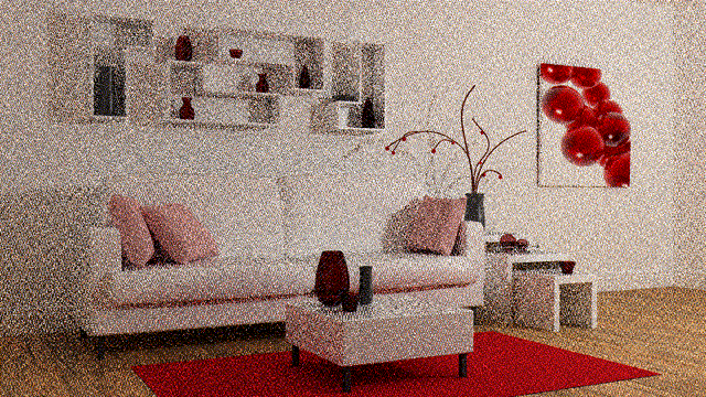
如果认为,以路径追踪的方式,计算一次一着色点的直接光照和一次弹射的间接光照 为 1 sample per pixel (1 SPP)。那么对于一帧,即使是 RTX 系列的 GPU 也只能做到 1 SPP,此时的噪声会非常夸张。但是路径追踪依旧为我们提供了非常宝贵的间接光照信息,那么接下来工作的重心就在如何降噪上了。降噪分为两个部分,单帧降噪与像素在时间上的复用。
单帧降噪
双边滤波
与其他滤波方式类似,双边滤波也使用周围像素的加权平均值代替中心像素值。重要的是双边滤波的权重不仅考虑了像素的欧氏距离(比如高斯滤波只考虑距离对权值的影响),还考虑了滤波范围域中的辐射差异。
w ( i , j , k , l ) = e x p ( − ( i − k ) 2 + ( j − l ) 2 2 σ d 2 − ∣ I ( i , j ) − I ( k , l ) ∣ 2 2 σ r 2 ) w(i,j,k,l)=exp(-\frac{(i-k)^2+(j-l)^2}{2\sigma _d^2}-\frac{|I(i,j)-I(k,l)|^2}{2\sigma _r^2}) w ( i , j , k , l ) = e x p ( − 2 σ d 2 ( i − k ) 2 + ( j − l ) 2 − 2 σ r 2 ∣ I ( i , j ) − I ( k , l ) ∣ 2 )
联合双边滤波
既然现在是在图形学中进行滤波,那么我们可以很轻易地从渲染管线中扒拉出更多有参考价值的信息,比如说任意像素的深度信息、世界坐标、法线方向等,甚至为不同的物体进行编号,只要将这些信息存在一张 Buffer 中即可。
J ( i , j ) = e x p ( − ∣ i − j ∣ 2 2 σ p 2 − ∣ C ~ [ i ] − C ~ [ j ] ∣ 2 2 σ c 2 − D n o r m a l ( i , j ) 2 2 σ n 2 − D p l a n e ( i , j ) 2 2 σ d 2 ) J(i,j)=exp(-\frac{|i-j|^2}{2\sigma _p^2}-\frac{|\widetilde{C}[i]-\widetilde{C}[j]|^2}{2\sigma _c^2}-\frac{D_{normal}(i,j)^2}{2\sigma _n^2}-\frac{D_{plane}(i,j)^2}{2\sigma _d^2}) J ( i , j ) = e x p ( − 2 σ p 2 ∣ i − j ∣ 2 − 2 σ c 2 ∣ C [ i ] − C [ j ] ∣ 2 − 2 σ n 2 D n or ma l ( i , j ) 2 − 2 σ d 2 D pl an e ( i , j ) 2 )
其中:
C ~ \widetilde{C} C D n o r m a l ( i , j ) = a r c c o s ( N o r m a l [ i ] ⋅ N o r m a l [ j ] ) D_{normal}(i,j)=arccos(Normal[i]\cdot Normal[j]) D n or ma l ( i , j ) = a rccos ( N or ma l [ i ] ⋅ N or ma l [ j ]) D p l a n e ( i , j ) = N o r m a l [ i ] ⋅ P o s i t i o n [ i ] − P o s i t i o n [ i ] ∣ P o s i t i o n [ j ] − P o s i t i o n [ i ] D_{plane}(i,j)=Normal[i]\cdot \frac{Position[i]-Position[i]}{|Position[j]-Position[i]} D pl an e ( i , j ) = N or ma l [ i ] ⋅ ∣ P os i t i o n [ j ] − P os i t i o n [ i ] P os i t i o n [ i ] − P os i t i o n [ i ]
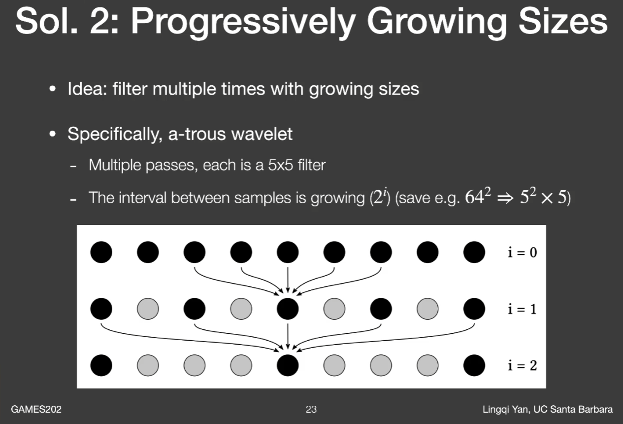
假如要遍历完 NxN 个像素会是一个较大的性能开销,这里使用 a-trous wavelet transform 的方式加速采样滤波核内的像素。每一趟固定采样 5x5 个像素,第 i 趟时采样点之间的距离为 2 i − 1 2^{i-1} 2 i − 1 o ( n 2 ) o(n^2) o ( n 2 ) o ( l o g 2 n ) o(log _2n) o ( l o g 2 n )
实现
1
2
3
4
5
6
7
8
9
10
11
12
13
14
15
16
17
18
19
20
21
22
23
24
25
26
27
28
29
30
31
32
33
34
35
36
37
38
39
40
41
42
43
44
45
46
47
48
49
50
51
52
53
54
55
56
57
58
59
60
61
62
63
64
65
66
67
68
69
70
71
72
73
74
75
76
77
78
79
80
81
82
83
84
85
86
87
88
89
90
91
92
93
94
95
96
97
98
99
100
101
102
103
104
105
106
107
108
109
110
111
112
113
114
115
116
117
118
119
120
121
122
123
124
125
126
127
128
129
130
131
132
133
134
float DistanceDifPow (int i_x, int i_y, int j_x, int j_y) return float (pow ((i_x - j_x), 2 ) + pow ((i_y - j_y), 2 ));float CloorDifPow (Float3 color_i, Float3 color_j) return dif.x * dif.x + dif.y * dif.y + dif.z * dif.z;float DnormalPow (Float3 normal_i, Float3 normal_j) float cosTerm = std::clamp (Dot (normal_i, normal_j), 0.f , 1.f );float acos = std::acos (cosTerm);return pow (acos, 2 );float DplanePow (Float3 normal_i, Float3 position_i, Float3 position_j) Normalize (position_j - position_i);return std::clamp ((float )pow (Dot (normal_i, nor), 2 ), 1e-5f , 1.f );float JointBilateralFilteringKernel (float distanceDifPow, float colorDifPow, float normalDifPow, float positionDifPow, float sigma_p, float sigma_c, float sigma_n, float sigma_d) return exp (-(distanceDifPow / (2 * pow (sigma_p, 2 ))) -2 * pow (sigma_c, 2 ))) -2 * pow (sigma_n, 2 ))) -2 * pow (sigma_d, 2 ))));Buffer2D<Float3> Denoiser::Filter (const FrameInfo &frameInfo) {int height = frameInfo.m_beauty.m_height;int width = frameInfo.m_beauty.m_width;int kernelRadius = 16 ;CreateBuffer2D <Float3>(width, height);CreateBuffer2D <Float3>(width, height);CreateBuffer2D <Float3>(width, height);CreateBuffer2D <Float3>(width, height);#pragma omp parallel for for (int y = 0 ; y < height; y++) {for (int x = 0 ; x < width; x++) {filteredImage (x, y) = frameInfo.m_beauty (x, y);imageBuffer (x, y) = frameInfo.m_beauty (x, y);normalBuffer (x, y) = frameInfo.m_normal (x, y);positionBuffer (x, y) = frameInfo.m_position (x, y);float weight = 0.f ;int step = 1 ;bool useA_trou = true ;if (useA_trou) {for (int num = 0 ; 2 * step <= kernelRadius; num++) {pow (2 , num);for (int j_y = y - 2 * step; j_y <= y + 2 * step; j_y += step) {for (int j_x = x - 2 * step; j_x <= x + 2 * step; j_x += step) {if (j_y < 0 || j_y >= height || j_x < 0 || j_x >= width) {continue ;imageBuffer (j_x, j_y) = frameInfo.m_beauty (j_x, j_y);normalBuffer (j_x, j_y) = frameInfo.m_normal (j_x, j_y);positionBuffer (j_x, j_y) = frameInfo.m_position (j_x, j_y);float distanceTerm = DistanceDifPow (x, y, j_x, j_y);float colorTerm =CloorDifPow (imageBuffer (x, y), imageBuffer (j_x, j_y));float normalTerm =DnormalPow (normalBuffer (x, y), normalBuffer (j_x, j_y));float planeTerm =DplanePow (normalBuffer (x, y),positionBuffer (x, y), positionBuffer (j_x, j_y));if (width >= 1280 ) {20 ;float exp = JointBilateralFilteringKernel (filteredImage (x, y) += imageBuffer (j_x, j_y) * exp;else {for (int j_y = y - kernelRadius; j_y <= y + kernelRadius; ++j_y) {for (int j_x = x - kernelRadius; j_x <= x + kernelRadius; ++j_x) {if (j_y < 0 || j_y >= height || j_x < 0 || j_x >= width) {continue ;imageBuffer (j_x, j_y) = frameInfo.m_beauty (j_x, j_y);normalBuffer (j_x, j_y) = frameInfo.m_normal (j_x, j_y);positionBuffer (j_x, j_y) = frameInfo.m_position (j_x, j_y);float distanceTerm = DistanceDifPow (x, y, j_x, j_y);float colorTerm =CloorDifPow (imageBuffer (x, y), imageBuffer (j_x, j_y));float normalTerm =DnormalPow (normalBuffer (x, y), normalBuffer (j_x, j_y));float planeTerm =DplanePow (normalBuffer (x, y),positionBuffer (x, y), positionBuffer (j_x, j_y));if (width >= 1280 ) { 30 ;float exp = JointBilateralFilteringKernel (filteredImage (x, y) += imageBuffer (j_x, j_y) * exp;if (weight > 0.f ) {filteredImage (x, y) /= weight;else {filteredImage (x, y) = 0.f ;return filteredImage;
结果
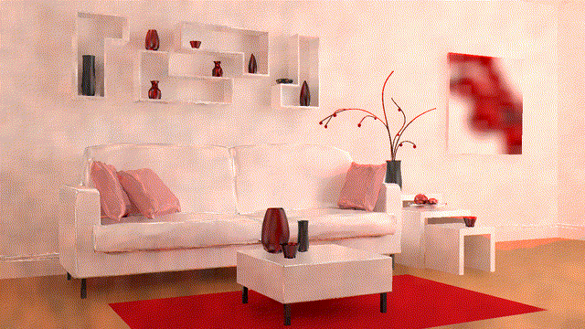
滤波之后亮度提高的原因 :事实上第二张图的亮度并没有提高,第一张图的辐射期望也是正确的。第一张图的亮度看起来偏暗是由于路径追踪的方差过大,以至于有大量超过 RGB 色域显示范围的 Irradiance 被直接 Clamp 至 255,产生了能量损失。在第二张图中进行滤波便是将无法显示的数值分配给了周围的像素,使得这部分数值可以正常地被显示出来。
时间上的累积
先将当前帧做单帧滤波,然后把一像素点在上一帧所在位置的像素值按一定权值混合入当前帧。如果说每一帧都能做 1 SPP,那么便几乎相当于一秒内将 30 SPP 的采样结果累积了下来。
投影到上一帧
第一个问题,如何找到一像素点在上一帧所对应的位置,准确来说是:一像素点对应世界坐标变换回上一帧的世界坐标,然后变换至上一帧的屏幕空间的坐标。
S c r e e n i − 1 = P i − 1 V i − 1 M i − 1 M i − 1 W o r l d i Screen_{i-1}=P_{i-1}V_{i-1}M_{i-1}M_i^{-1}World_i S cree n i − 1 = P i − 1 V i − 1 M i − 1 M i − 1 W or l d i
其中:
下角标的 i 代表第 i 帧
M 代表物体坐标系到世界坐标系的矩阵
V 代表世界坐标系到摄像机坐标系的矩阵
P 代表摄像机坐标系到屏幕坐标系的矩阵
得到上一帧的屏幕空间坐标后需要检查:
上一帧是否在屏幕内。(该点第一次出现于屏幕内,没有时间上的信息)
上一帧和当前帧的物体的标号。(该点上一帧被另一物体遮挡,不应当使用时间上的信息)
若坐标非法便不使用上一帧的数据,100% 使用当前帧的数据。投影坐标的合法性保存在 m_valid 中供下一步参考。
实现
1
2
3
4
5
6
7
8
9
10
11
12
13
14
15
16
17
18
19
20
21
22
23
24
25
26
27
28
29
30
31
32
33
34
35
36
37
38
39
40
41
42
43
44
void Denoiser::Reprojection (const FrameInfo& frameInfo) int height = m_accColor.m_height;int width = m_accColor.m_width;size () - 1 ];#pragma omp parallel for for (int y = 0 ; y < height; y++) {for (int x = 0 ; x < width; x++) {int id = (int )frameInfo.m_id (x, y);if (-1 != id) {Inverse (frameInfo.m_matrix[id]);PVMM_1 (frameInfo.m_position (x, y), Float3::Point);int pre_x = (int )projPos.x;int pre_y = (int )projPos.y;if (pre_x < 0 || pre_x >= width || pre_y < 0 || pre_y >= height) {m_valid (x, y) = false ;continue ;int pre_id = (int )m_preFrameInfo.m_id (pre_x, pre_y);if (pre_id != id) {m_valid (x, y) = false ;continue ;m_misc (x, y) = m_accColor (pre_x, pre_y);m_valid (x, y) = true ;swap (m_misc, m_accColor);
混合入当前帧
将已降噪的当前帧C ‾ i \overline{C}_i C i C ‾ i − 1 \overline{C}_{i-1} C i − 1
C ‾ i = α C ‾ i + ( 1 − α ) C l a m p ( C ‾ i − 1 ) \overline{C}_i=\alpha \overline{C}_i+(1-\alpha)Clamp(\overline{C}_{i-1}) C i = α C i + ( 1 − α ) Cl am p ( C i − 1 )
如果上一帧的坐标非法,α \alpha α
Clamp
计算 C ‾ i \overline{C}_i C i μ \mu μ σ \sigma σ ( μ − k σ , μ + k σ ) (\mu -k\sigma,\mu +k\sigma) ( μ − kσ , μ + kσ )
实现
1
2
3
4
5
6
7
8
9
10
11
12
13
14
15
16
17
18
19
20
21
22
23
24
25
26
27
28
29
30
31
32
33
34
35
36
37
38
39
40
41
42
43
44
45
46
47
void Denoiser::TemporalAccumulation (const Buffer2D<Float3> &curFilteredColor) int height = m_accColor.m_height;int width = m_accColor.m_width;int range = 2 ;#pragma omp parallel for for (int y = 0 ; y < height; y++) {for (int x = 0 ; x < width; x++) {m_accColor (x, y);Float3 mu (0.f ) ;for (int i = x - range; i <= x + range; i++) {for (int j = y - range; j <= y + range; j++) {curFilteredColor (i, j);float )pow (2.f * range + 1.f , 2 );Float3 sigma (0.f ) ;for (int i = x - range; i <= x + range; i++) {for (int j = y - range; j <= y + range; j++) {Sqr (curFilteredColor (i, j) - mu);float )pow (2.f * range + 1.f , 2 );if (width >= 1280 ) {0.1f ;Clamp (preColor,float alpha = 1.0f ;if (m_valid (x, y)) {m_misc (x, y) = Lerp (preColor, curFilteredColor (x, y), alpha);swap (m_misc, m_accColor);
结果