本文最后更新于 2025-03-09T19:44:04+08:00
渲染管线中的变换矩阵
在渲染管线的前期,光栅化之前,需要对顶点和相机的坐标进行标准化变换,然后进行视口变换进入屏幕坐标空间。
相机的定义
位置:e ⃗ \vec{e} e g ⃗ \vec{g} g t ⃗ \vec{t} t
我们规定相机位于 (0, 0, 0) ,看向 -Z,上方为 Y。
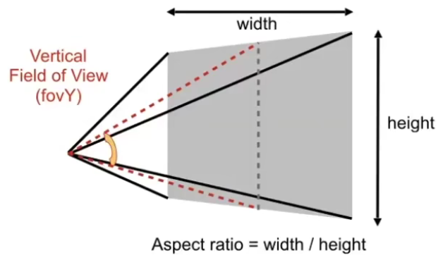
视锥体的定义
t a n f o v Y 2 = t ∣ n ∣ tan\frac{fovY}{2} = \frac{t}{|n|} t an 2 f o v Y = ∣ n ∣ t a s p e c t = r t aspect = \frac{r}{t} a s p ec t = t r
像素空间
像素块编号 (0, 0) -> (width - 1, height - 1)
Viewing
Model-View
M v i e w = R v i e w T v i e w M_{view}=R_{view}T_{view} M v i e w = R v i e w T v i e w T v i e w = T_{view}= T v i e w =
( 1 0 0 − x e 0 1 0 − y e 0 0 1 − z e 0 0 0 1 ) \begin{pmatrix}
1 & 0 & 0 & -x_e \\
0 & 1 & 0 & -y_e \\
0 & 0 & 1 & -z_e \\
0 & 0 & 0 & 1 \\
\end{pmatrix}
1 0 0 0 0 1 0 0 0 0 1 0 − x e − y e − z e 1
R v i e w − 1 R_{view}^{-1} R v i e w − 1
将 X(1,0,0)旋转至(g x t),将 Y(0,1,0)旋转至 t,将 Z(0,0,1)旋转至 -g。
由 R v i e w − 1 = R_{view}^{-1}= R v i e w − 1 =
( x g × t x t x − g 0 y g × t y t y − g 0 z g × t z t z − g 0 0 0 0 1 ) \begin{pmatrix}
x_{g \times t} & x_t & x_{-g} & 0 \\
y_{g \times t} & y_t & y_{-g} & 0 \\
z_{g \times t} & z_t & z_{-g} & 0 \\
0 & 0 & 0 & 1 \\
\end{pmatrix}
x g × t y g × t z g × t 0 x t y t z t 0 x − g y − g z − g 0 0 0 0 1
得 R v i e w = R_{view}= R v i e w =
( x g × t y g × t z g × t 0 x t y t z t 0 x − g y − g z − g 0 0 0 0 1 ) \begin{pmatrix}
x_{g \times t} & y_{g \times t} & z_{g \times t} & 0 \\
x_t & y_t & z_t & 0 \\
x_{-g} & y_{-g} & z_{-g} & 0 \\
0 & 0 & 0 & 1 \\
\end{pmatrix}
x g × t x t x − g 0 y g × t y t y − g 0 z g × t z t z − g 0 0 0 0 1
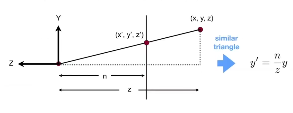
Projection
Persprctive to Orthographic
y , = n z y y^, = \frac{n}{z}y y , = z n y x , = n z x x^, = \frac{n}{z}x x , = z n x
在齐次坐标系下,对一个坐标的所有元素乘以或除以同一个数仍然代表原本的坐标。
故 一点 ( x , y , z , 1 ) T (x,y,z,1)^T ( x , y , z , 1 ) T M p 2 o M_{p2o} M p 2 o
( n x z n y z ? 1 ) \begin{pmatrix}
\frac{nx}{z} \\
\frac{ny}{z} \\
? \\
1 \\
\end{pmatrix}
z n x z n y ? 1
即:
( n x n y ? z ) \begin{pmatrix}
nx \\
ny \\
? \\
z \\
\end{pmatrix}
n x n y ? z
所以:M p 2 o = M_{p2o} = M p 2 o =
( n 0 0 0 0 n 0 0 ? ? ? ? 0 0 1 0 ) \begin{pmatrix}
n & 0 & 0 & 0 \\
0 & n & 0 & 0 \\
? & ? & ? & ? \\
0 & 0 & 1 & 0 \\
\end{pmatrix}
n 0 ? 0 0 n ? 0 0 0 ? 1 0 0 ? 0
又因为 f、n 平面在变换后 z 轴不变,( x , y , n , 1 ) T (x,y,n,1)^T ( x , y , n , 1 ) T ( ? , ? , ? , ? ) (?,?,?,?) ( ? , ? , ? , ?) n 2 n^2 n 2
( ? , ? , ? , ? ) = ( 0 , 0 , A , B ) (?,?,?,?)=(0,0,A,B) ( ? , ? , ? , ?) = ( 0 , 0 , A , B ) A n + B = n 2 An+B=n^2 A n + B = n 2
且远平面上中心点 ( 0 , 0 , f , 1 ) T (0,0,f,1)^T ( 0 , 0 , f , 1 ) T ( 0 , 0 , A , B ) (0,0,A,B) ( 0 , 0 , A , B ) f 2 f^2 f 2
联立得:
( 0 , 0 , A , B ) = ( 0 , 0 , n + f , − n f ) (0,0,A,B)=(0,0,n+f,-nf) ( 0 , 0 , A , B ) = ( 0 , 0 , n + f , − n f )
综上所述,M p 2 o = M_{p2o}= M p 2 o =
( n 0 0 0 0 n 0 0 0 0 n + f − n f 0 0 1 0 ) \begin{pmatrix}
n & 0 & 0 & 0 \\
0 & n & 0 & 0 \\
0 & 0 & n+f & -nf \\
0 & 0 & 1 & 0 \\
\end{pmatrix}
n 0 0 0 0 n 0 0 0 0 n + f 1 0 0 − n f 0
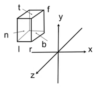
Orthographic
将裁剪空间转化为标准化设备坐标,中心为 (0, 0, 0),大小为 1x1x1 的立方体。
M o r t h o = M_{ortho}= M or t h o =
( 2 r − l 0 0 − r + l 2 0 2 t − b 0 − t + b 2 0 0 2 n − f − n + f 2 0 0 0 1 ) \begin{pmatrix}
\frac{2}{r-l} & 0 & 0 & -\frac{r+l}{2} \\
0 & \frac{2}{t-b} & 0 & -\frac{t+b}{2} \\
0 & 0 & \frac{2}{n-f} & -\frac{n+f}{2} \\
0 & 0 & 0 & 1 \\
\end{pmatrix}
r − l 2 0 0 0 0 t − b 2 0 0 0 0 n − f 2 0 − 2 r + l − 2 t + b − 2 n + f 1
Projection
M P r o j e c t i o n = M O r t h o g r a p h i c M P e r s p r c t i v e T o O r t h o g r a p h i c M_{Projection}=M_{Orthographic}M_{PersprctiveToOrthographic} M P ro j ec t i o n = M O r t h o g r a p hi c M P ers p rc t i v e T o O r t h o g r a p hi c
Viewport
先将标准化设备坐标拉伸至与屏幕同等大小,再将其中心 (0, 0) 移至屏幕中心。保留 z 轴不变用于之后做深度检测。M v i e w p o r t = M_{viewport}= M v i e wp or t =
( w i d t h 2 0 0 w i d t h 2 0 h e i g h t 2 0 h e i g h t 2 0 0 1 0 0 0 0 1 ) \begin{pmatrix}
\frac{width}{2} & 0 & 0 & \frac{width}{2} \\
0 & \frac{height}{2} & 0 & \frac{height}{2} \\
0 & 0 & 1 & 0 \\
0 & 0 & 0 & 1 \\
\end{pmatrix}
2 w i d t h 0 0 0 0 2 h e i g h t 0 0 0 0 1 0 2 w i d t h 2 h e i g h t 0 1
Super Sample Anti-Aliasing
SSAA 作为一种暴力的超采样手段带来的性能开销是难以接受的,但作为反走样的入门仍然有学习的必要。
insideTriangle
判断两向量的左右关系
假设两向量 a ⃗ \vec{a} a b ⃗ \vec{b} b a ⃗ × b ⃗ \vec{a} \times \vec{b} a × b b ⃗ \vec{b} b a ⃗ \vec{a} a
那么对于三角形三点形成的顺 \ 逆时针三条向量来说,若有一点同时位于三向量的同一侧,则该点位于三角形内部。
假设三角形三点 a、b、c 与点 p 在同一平面上。a b ⃗ \vec{ab} ab b c ⃗ \vec{bc} b c c a ⃗ \vec{ca} c a a p ⃗ \vec{ap} a p b p ⃗ \vec{bp} b p c p ⃗ \vec{cp} c p
1
2
3
4
5
6
7
8
9
10
11
12
13
14
15
16
17
18
19
20
21
static bool insideTriangle (float x, float y, const Vector3f* _v) Eigen::Vector3f p (x, y, 0 ) ;Eigen::Vector3f a (_v[0 ][0 ], _v[0 ][1 ], 0 ) ;Eigen::Vector3f b (_v[1 ][0 ], _v[1 ][1 ], 0 ) ;Eigen::Vector3f c (_v[2 ][0 ], _v[2 ][1 ], 0 ) ;cross (ap);cross (bp);cross (cp);return ((crs1[2 ] >= 0 && crs2[2 ] >= 0 && crs3[2 ] >= 0 ) ||2 ] <= 0 && crs2[2 ] <= 0 && crs3[2 ] <= 0 ));
SSAA & zBuffer
遍历包围盒内的像素,对于每个像素遍历每个超采样点,确定三角形覆盖像素的比例,通过重心坐标计算对应的深度值,与深度缓存做比较并写入帧缓存。
1
2
3
4
5
6
7
8
9
10
11
12
13
14
15
16
17
18
19
20
21
22
23
24
25
26
27
28
29
30
31
32
33
34
35
36
37
38
39
40
41
42
43
44
45
46
47
48
49
50
51
52
53
54
55
56
57
58
59
void rst::rasterizer::rasterize_triangle (const Triangle& t) {auto v = t.toVector4 ();int minX = (int )std::floor (std::min (v[0 ][0 ], std::min (v[1 ][0 ], v[2 ][0 ])));int maxX = (int )std::ceil (std::max (v[0 ][0 ], std::max (v[1 ][0 ], v[2 ][0 ])));int minY = (int )std::floor (std::min (v[0 ][1 ], std::min (v[1 ][1 ], v[2 ][1 ])));int maxY = (int )std::ceil (std::max (v[0 ][1 ], std::max (v[1 ][1 ], v[2 ][1 ])));0.25f ,0.25f },0.75f ,0.25f },0.25f ,0.75f },0.75f ,0.75f },for (int x = minX; x <= maxX; x++) {for (int y = minY; y <= maxY; y++) {int insideCount = 0 ;float sumDepth = 0.f ;for (int i = 0 ; i < 4 ; i++) {if (insideTriangle ((float )x + super[i][0 ],float )y + super[i][1 ], t.v)) {auto tup = computeBarycentric2D (float )x + super[i][0 ], (float )y + super[i][1 ], t.v);float alpha, beta, gamma;tie (alpha, beta, gamma) = tup;float w_reciprocal = 1.f /0 ].w () + beta / v[1 ].w () + gamma / v[2 ].w ());float z_interpolated = alpha * v[0 ].z () / v[0 ].w () +1 ].z () / v[1 ].w () + gamma * v[2 ].z () / v[2 ].w ();if (insideCount > 0 ) {float avgDepth = sumDepth / 4.f ;if (avgDepth < depth_buf[get_index (x, y)]) {get_index (x, y)] = avgDepth;Eigen::Vector3f point ((float )x, (float )y, avgDepth) ;getColor () * insideCount / 4.f ;set_pixel (point, color);
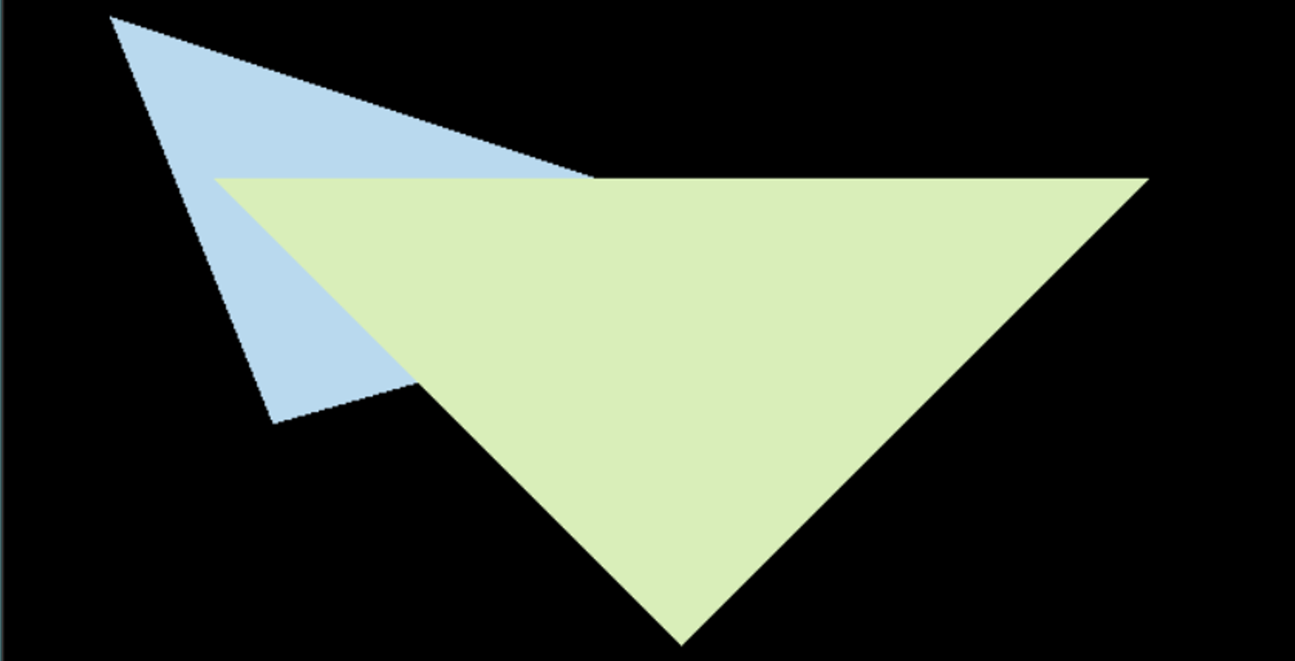
结果
Blinn-Phong 光照模型
该模型将任一点的光照分为三部分:1.由光源方向与法线方向决定的漫反射、2.由光源方向法线方向与观察方向决定的高光、3.恒定的环境光。
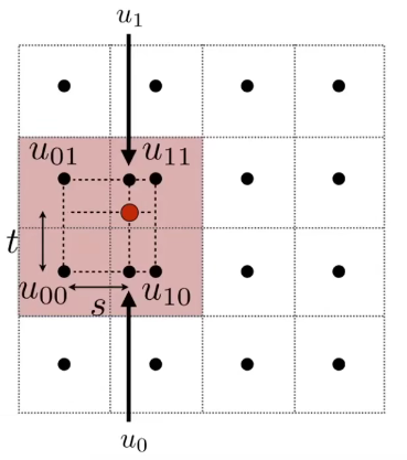
getColorBilinear
1
2
3
4
5
6
7
8
9
10
11
12
13
14
15
16
17
18
19
20
21
22
23
24
25
26
27
28
Eigen::Vector3f getColorBilinear (float u, float v) {if (u > 1 ) u = u - (int )u;if (u < 0 ) u = u - (int )u + 1 ;if (v > 1 ) v = v - (int )v;if (v < 0 ) v = v - (int )v + 1 ;float u_img = u * width;float v_img = (1 - v) * height;int u_min = (int )std::floor (u_img);int u_max = (int )std::min ((float )width, std::ceil (u_img));int v_min = (int )std::floor (v_img);int v_max = (int )std::min ((float )height, std::ceil (v_img));auto u00 = image_data.at <cv::Vec3b>(v_min, u_min);auto u01 = image_data.at <cv::Vec3b>(v_max, u_min);auto u10 = image_data.at <cv::Vec3b>(v_min, u_max);auto u11 = image_data.at <cv::Vec3b>(v_max, u_max);float s = (u_img - u_min) / (u_max - u_min);float t = (v_img - v_min) / (v_max - v_min);auto u0 = (1 - s) * u00 + s * u10;auto u1 = (1 - s) * u01 + s * u11;auto p = (1 - t) * u0 + t * u1;return Eigen::Vector3f (p[0 ], p[1 ], p[2 ]);
布林-冯
1
2
3
4
5
6
7
8
9
10
11
12
13
14
15
16
17
18
19
20
21
22
23
24
25
26
27
28
29
30
31
32
33
34
35
36
37
38
39
40
41
42
43
44
45
46
47
48
49
50
51
52
53
54
55
56
Eigen::Vector3f texture_fragment_shader (const fragment_shader_payload& payload) {Identity ();bool isBilinear = true ;if (payload.texture) {if (isBilinear) {getColorBilinear (x (), payload.tex_coords.y ());else {getColor (x (), payload.tex_coords.y ());255.f ;Vector3f (0.7937f , 0.7937f , 0.7937f );Vector3f (0.01f , 0.01f , 0.01f );auto l1 = light{ {20 , 20 , 20 }, {500 , 500 , 500 } };auto l2 = light{ {-20 , 20 , 0 }, {500 , 500 , 500 } };float p = 200.0f ;10 , 10 , 10 };0 , 0 , 10 };0 , 0 , 0 };for (auto & light : lights) {float r2 = lightVector.dot (lightVector);cwiseProduct (light.intensity) / r2 *max (0.f , normal.dot (lightVector.normalized ()));normalized () + lightVector.normalized ();norm ();cwiseProduct (light.intensity) / r2 *pow (std::max (0.f , normal.dot (h)), p);cwiseProduct (amb_light_intensity);return result_color * 255.f ;
结果
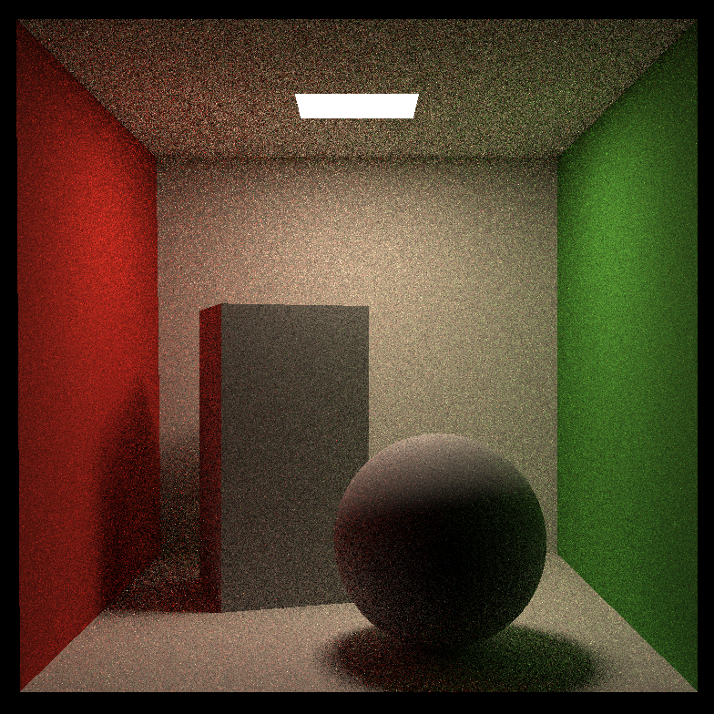
Whitted-Style 光线追踪
Whitted_Style 光线追踪的部分实现,包括射线与由重心坐标表式的三角形相交、射线与轴对齐包围盒的相交、包围盒的树形加速结构。
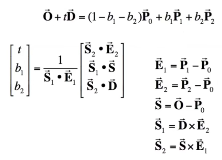
Möller-Trumbore 射线与平面(重心坐标)
光线的定义:
O ⃗ + t D ⃗ \vec{O}+t\vec{D} O + t D
平面的定义:
( 1 − b 1 − b 2 ) P ⃗ 0 + b 1 P ⃗ 1 + b 2 P ⃗ 2 (1-b_1-b_2)\vec{P}_0+b_1\vec{P}_1+b_2\vec{P}_2 ( 1 − b 1 − b 2 ) P 0 + b 1 P 1 + b 2 P 2
求射线与平面的交点即联立两表达式求解,已知 xyz 三分量上的三对表达式,求未知量:t、b 1 b_1 b 1 b 2 b_2 b 2
对于用重心坐标表示的三角形,三值之和为 1 即可表示当前平面上的任一点,若同时三值均大于 1 则表示该三角形内部的一点。
1
2
3
4
5
6
7
8
9
10
11
12
13
14
15
16
17
18
bool rayTriangleIntersect (const Vector3f& v0, const Vector3f& v1, const Vector3f& v2, const Vector3f& orig, const Vector3f& dir) crossProduct (dir, e2);crossProduct (s, e1);float factor = dotProduct (s1, e1);float t = dotProduct (s2, e2) / factor;float b1 = dotProduct (s1, s) / factor;float b2 = dotProduct (s2, dir) / factor;if (t >= 0 && b1 >= 0 && b2 >= 0 && (1 - b1 - b2) >= 0 )return true ;return false ;
射线与平面(点法式)
平面的定义:
( P ⃗ − P , ⃗ ) ⋅ N ⃗ (\vec{P}-\vec{P^,})\cdot \vec{N} ( P − P , ) ⋅ N
点 P , P^, P ,
t = ( P , ⃗ − O ⃗ ) ⋅ N ⃗ D ⃗ ⋅ N ⃗ t=\frac{(\vec{P^,}-\vec{O})\cdot \vec{N}}{\vec{D}\cdot \vec{N}} t = D ⋅ N ( P , − O ) ⋅ N
射线与轴对齐包围盒
包围盒的定义:pMax 与 pMin 两个点所代表的三对面。
t = P x , ⃗ − O x ⃗ D x ⃗ t=\frac{\vec{P^,_x}-\vec{O_x}}{\vec{D_x}} t = D x P x , − O x
对于每一对平面,射线存在一对与他们相交的 t m i n t_{min} t min t m a x t_{max} t ma x
t e n t e r = m a x ( t m i n ) t_{enter}=max(t_{min}) t e n t er = ma x ( t min ) t e x i t = m i n ( t m a x ) t_{exit}=min(t_{max}) t e x i t = min ( t ma x )
射线与包围盒有一段相交:t e n t e r < t e x i t t_{enter}<t_{exit} t e n t er < t e x i t
1 2 3 4 5 6 7 8 9 10 11 12 13 14 15 16 17 18 19 20 21 22 23 24 25 26 27 28 #include <limits> inline bool Bounds3::IntersectP (const Ray& ray, const Vector3f& invDir, const std::array<bool , 3 >& dirIsNeg) const float tEnter = std::numeric_limits<float >::lowest ();float tExit = std::numeric_limits<float >::max ();for (int i = 0 ; i < 3 ; i++) {float tMin = (pMin[i] - ray.origin[i]) * invDir[i];float tMax = (pMax[i] - ray.origin[i]) * invDir[i];if (dirIsNeg[i]) {swap (tMin, tMax);if (tMin > tEnter) {if (tMax < tExit) {return (tEnter < tExit && tExit >= 0 );
BVH 的创建
轴对齐包围盒的加速结构
1
2
3
4
5
6
7
8
9
10
11
12
13
14
15
16
17
18
19
20
21
22
23
24
25
26
27
28
29
30
31
32
33
34
35
36
37
38
39
40
41
42
43
44
45
46
47
48
49
50
51
52
53
54
55
56
57
58
59
60
61
62
63
64
65
BVHBuildNode* BVHAccel::recursiveBuild (std::vector<Object*> objects) {new BVHBuildNode ();for (int i = 0 ; i < objects.size (); ++i)Union (bounds, objects[i]->getBounds ());if (objects.size () == 1 ) {0 ]->getBounds ();0 ];nullptr ;nullptr ;return node;else if (objects.size () == 2 ) {recursiveBuild (std::vector{objects[0 ]});recursiveBuild (std::vector{objects[1 ]});Union (node->left->bounds, node->right->bounds);return node;else {for (int i = 0 ; i < objects.size (); ++i)Union (centroidBounds, objects[i]->getBounds ().Centroid ());int dim = centroidBounds.maxExtent ();switch (dim) {case 0 :sort (objects.begin (), objects.end (), [](auto f1, auto f2) {return f1->getBounds ().Centroid ().x <getBounds ().Centroid ().x;break ;case 1 :sort (objects.begin (), objects.end (), [](auto f1, auto f2) {return f1->getBounds ().Centroid ().y <getBounds ().Centroid ().y;break ;case 2 :sort (objects.begin (), objects.end (), [](auto f1, auto f2) {return f1->getBounds ().Centroid ().z <getBounds ().Centroid ().z;break ;auto beginning = objects.begin ();auto middling = objects.begin () + (objects.size () / 2 );auto ending = objects.end ();auto leftshapes = std::vector <Object*>(beginning, middling);auto rightshapes = std::vector <Object*>(middling, ending);assert (objects.size () == (leftshapes.size () + rightshapes.size ()));recursiveBuild (leftshapes);recursiveBuild (rightshapes);Union (node->left->bounds, node->right->bounds);return node;
BVH 的创建(ASH)
表面积启发式算法基于两个假设:如果包围盒的表面积越大,那么它被射线击中的可能性也就越大。包围盒内的物体数量越多,遍历它的开销就越大。比较所有划分方案的预计开销并选择最优的方案。float cost = 1 + (countA * A.SurfaceArea() + countB * B.SurfaceArea()) / nArea;
1
2
3
4
5
6
7
8
9
10
11
12
13
14
15
16
17
18
19
20
21
22
23
24
25
26
27
28
29
30
31
32
33
34
35
36
37
38
39
40
41
42
43
44
45
46
47
48
49
50
51
52
53
54
55
56
57
58
59
60
61
62
63
64
65
66
67
68
69
70
71
72
73
74
75
76
77
78
79
80
81
82
83
84
85
86
87
88
89
90
91
92
93
94
95
96
97
98
99
100
101
102
103
104
105
106
107
108
109
110
111
112
BVHBuildNode* BVHAccel::recursiveBuild (std::vector<Object*> objects) {new BVHBuildNode ();for (int i = 0 ; i < objects.size (); ++i) {Union (bounds, objects[i]->getBounds ());if (objects.size () == 1 ) {0 ]->getBounds ();0 ];nullptr ;nullptr ;return node;else if (objects.size () == 2 ) {recursiveBuild (std::vector{objects[0 ]});recursiveBuild (std::vector{objects[1 ]});Union (node->left->bounds, node->right->bounds);return node;else {for (int i = 0 ; i < objects.size (); ++i) {Union (centroidBounds,objects[i]->getBounds ().Centroid ());for (int i = 0 ; i < objects.size (); ++i) {Union (nBounds, objects[i]->getBounds ());float nArea = centroidBounds.SurfaceArea ();int minCostCoor = 0 ;int mincostIndex = 0 ;float minCost = std::numeric_limits<float >::infinity ();int , std::map<int , int >> indexMap;for (int i = 0 ; i < 3 ; i++) {int bucketCount = 12 ;int > countBucket;for (int j = 0 ; j < bucketCount; j++) {push_back (Bounds3 ());push_back (0 );int , int > objMap;for (int j = 0 ; j < objects.size (); j++) {int bid = bucketCount * centroidBounds.Offset (getBounds ().Centroid ())[i];if (bid > bucketCount - 1 ) {1 ;Union (b, objects[j]->getBounds ().Centroid ());1 ;insert (std::make_pair (j, bid));insert (std::make_pair (i, objMap));for (int j = 1 ; j < boundsBuckets.size (); j++) {int countA = 0 ;int countB = 0 ;for (int k = 0 ; k < j; k++) {Union (A, boundsBuckets[k]);for (int k = j; k < boundsBuckets.size (); k++) {Union (B, boundsBuckets[k]);float cost = 1 + (countA * A.SurfaceArea () +SurfaceArea ()) / nArea;if (cost < minCost) {for (int i = 0 ; i < objects.size (); i++) {if (indexMap[minCostCoor][i] < mincostIndex) {push_back (objects[i]);else {push_back (objects[i]);assert (objects.size () == (leftshapes.size () + rightshapes.size ()));recursiveBuild (leftshapes);recursiveBuild (rightshapes);Union (node->left->bounds, node->right->bounds);return node;
BVH 的遍历
1
2
3
4
5
6
7
8
9
10
11
12
13
14
15
16
17
18
19
20
21
22
23
24
25
Intersection BVHAccel::getIntersection (BVHBuildNode* node, const Ray& ray) const {float x = ray.direction.x;float y = ray.direction.y;float z = ray.direction.z;bool , 3> dirsIsNeg{x < 0 ,y < 0 ,z < 0 };if (node->bounds.IntersectP (ray, ray.direction_inv, dirsIsNeg) == false ) {return inter;if (node->left == nullptr && node->right == nullptr ) {getIntersection (ray);return inter;getIntersection (node->left, ray);getIntersection (node->right, ray);if (hitL.distance < hitR.distance) {return hitL;return hitR;
结果
相关链接
参考
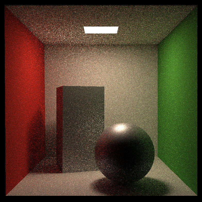
蒙特卡洛路径追踪
我们在上一章中得到了重要的渲染方程,在这一章中将使用蒙特卡洛算法实现方程中的积分,并用俄罗斯轮盘赌实现间接光照中对渲染方程的递归调用。
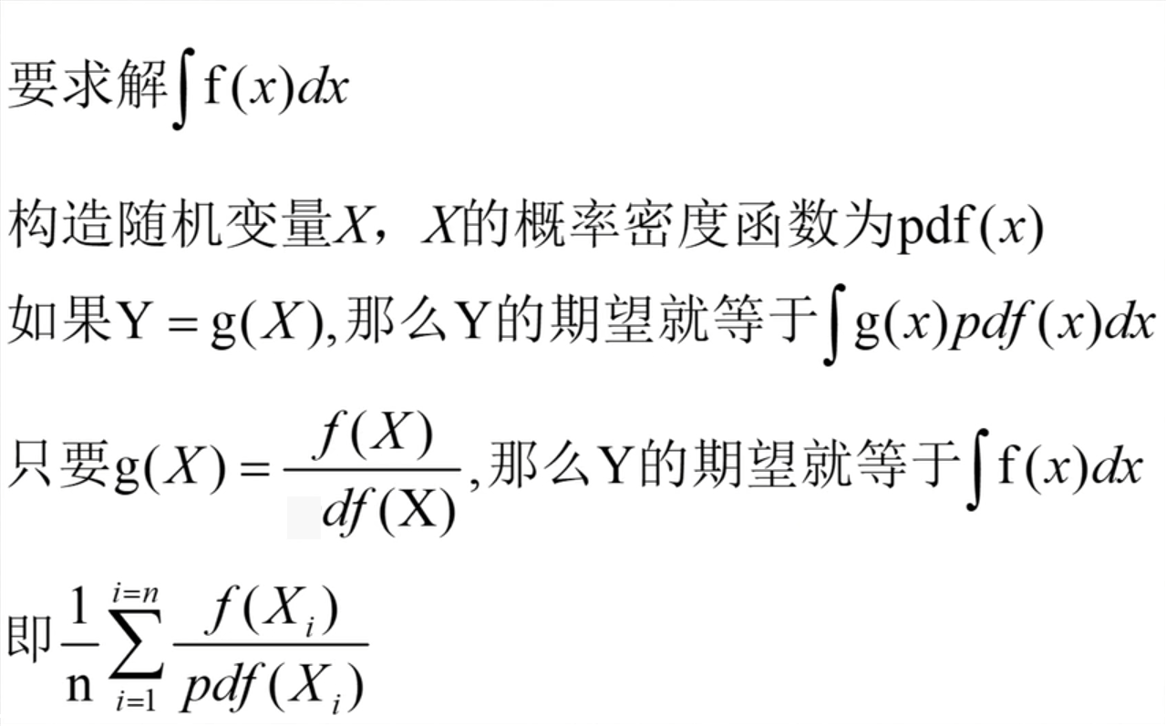
蒙特卡洛
按一定分布对原函数进行随机采样,利用概率分布函数进行加权平均。
∫ f ( x ) d x = 1 N ∑ i = 1 N f ( X i ) p , ( X i ) \int f(x){\rm d}x=\frac{1}{N}\sum^{N}_{i=1}\frac{f(X_i)}{p^,(X_i)} ∫ f ( x ) d x = N 1 ∑ i = 1 N p , ( X i ) f ( X i ) X i X_i X i p , ( x ) p^,(x) p , ( x ) L o ( p , ω o ) ≈ 1 N ∑ i = 1 N L i ( p , ω i ) f r ( p , ω i , ω o ) ( n ⋅ ω i ) p , ( ω i ) L_o(p,\omega_o)\approx \frac{1}{N}\sum^{N}_{i=1}\frac{L_i(p,\omega_i)f_r(p,\omega_i,\omega_o)(n\cdot \omega_i)}{p^,(\omega_i)} L o ( p , ω o ) ≈ N 1 ∑ i = 1 N p , ( ω i ) L i ( p , ω i ) f r ( p , ω i , ω o ) ( n ⋅ ω i ) p , ( ω i ) = π 2 p^,(\omega_i)=\frac{\pi}{2} p , ( ω i ) = 2 π
路径追踪
若计算每根光线反射出的N跟光线,递归次数呈指数级上涨,开销难以接受。解决方法 :对一个像素内多次发射出一根光线,每次反射只产生一根光线,结果求平均。此时上方的N = 1。
俄罗斯轮盘赌
接下来解决递归如何返回的问题。在真实世界中的光线可能会经过无数次弹射才进入人眼,但在有限的计算时间内这几乎是无法模拟的。解决方法 :以期望代替无限次递归逼近的结果。设一小数 p(0,1),每次递归内以概率 (p - 1) 直接返回 0,以概率 p 进入下一层递归,并对结果除以 p。此时递归的期望为:
E = P ∗ ( L o / P ) + ( 1 − P ) ∗ 0 = L o E=P*(L_o/P)+(1-P)*0=L_o E = P ∗ ( L o / P ) + ( 1 − P ) ∗ 0 = L o
递归的期望值确实是正确的,但是根据实现的不同,或者受制于显示器色域,超过 255 的值可能被截断至 255,导致结果看起来偏暗。
最后一个问题
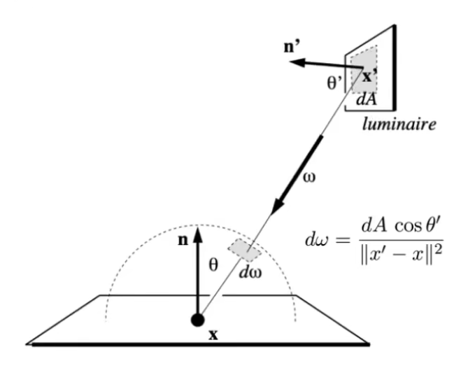
在目前的算法中,从视点发射出的一根光线若直到最终都没有击中发光物体便不会返回任何 Radiance。这样在场景中光源表面积非常小的情况下便很难产生有效的递归,因为对半球内方向随机采样难以精确采样到发光物体。解决方法 :每层递归内将直接光照与间接光照的贡献分离开,并直接对光源进行采样。这时需要将光源方向ω \omega ω 1 A \frac{1}{A} A 1
d ω = cos θ , d A ∣ x , − x ∣ 2 d\omega=\frac{\cos \theta^,dA}{|x^,-x|^2} d ω = ∣ x , − x ∣ 2 c o s θ , d A
可以理解为 cos θ , \cos \theta^, cos θ ,
L o ( x , ω o ) = ∫ A L i ( x , ω i ) f r ( x , ω i , ω o ) cos θ cos θ , ∣ x , − x ∣ 2 d A L_o(x,\omega_o)=\int_ALi(x,\omega_i)f_r(x,\omega_i,\omega_o)\frac{\cos \theta \cos \theta^,}{|x^,-x|^2}{\rm d}A L o ( x , ω o ) = ∫ A L i ( x , ω i ) f r ( x , ω i , ω o ) ∣ x , − x ∣ 2 c o s θ c o s θ , d A
伪代码
Shad(p, wo) {θ \theta θ θ , \theta^, θ , ∣ x , − p ∣ 2 |x^,-p|^2 ∣ x , − p ∣ 2 π \pi π cos θ \cos \theta cos θ
代码实现
1
2
3
4
5
6
7
8
9
10
11
12
13
14
15
16
17
18
19
20
21
22
23
24
25
26
27
28
29
30
31
32
33
34
35
36
37
38
39
40
41
42
43
44
45
46
47
48
49
50
51
52
53
54
55
56
57
58
59
60
61
62
63
64
65
Vector3f Scene::castRay (const Ray& ray, int depth) const {intersect (ray);if (inter.happened) {if (inter.m->hasEmission ()) {if (depth == 0 ) {return inter.m->getEmission ();else {return Vector3f (0 , 0 , 0 );Vector3f L_dir (0 , 0 , 0 ) ;Vector3f L_indir (0 , 0 , 0 ) ;float pdf_light = 0.f ;sampleLight (lightInter, pdf_light);normalized ();intersect (Ray (objPos, o2lDir));if (o2lInter.happened && o2lInter.m->hasEmission ()) {eval (ray.direction, o2lDir, N);dotProduct (o2lDir, N) * dotProduct (-o2lDir, NN) /dotProduct (objectToLight, objectToLight) / pdf_light;if (get_random_float () > RussianRoulette) {return Vector3f (0 , 0 , 0 );sample (ray.direction, N).normalized ();Ray nextRay (objPos, nextDir) ;intersect (nextRay);if (nextInter.happened && !nextInter.m->hasEmission ()) {float pdf_hemi = inter.m->pdf (ray.direction, nextDir, N);eval (ray.direction, nextDir, N);castRay (nextRay, depth + 1 ) * f_r * dotProduct (nextDir, N) /return L_dir + L_indir;return Vector3f (0 , 0 , 0 );
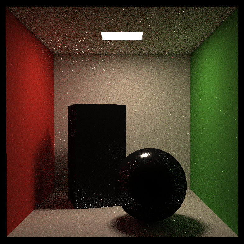
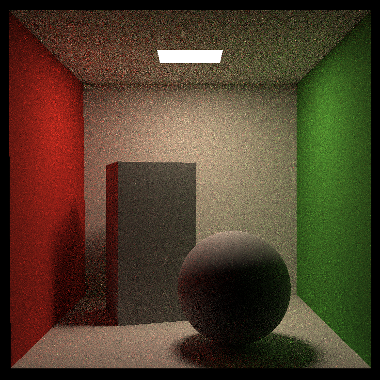
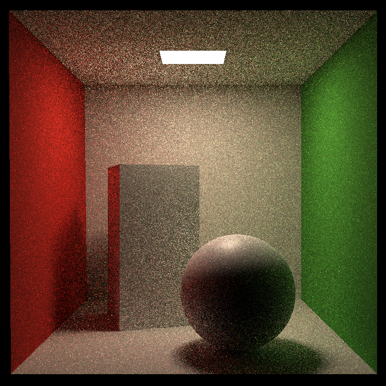
结果
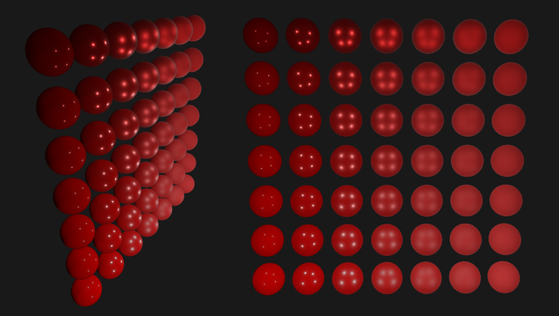
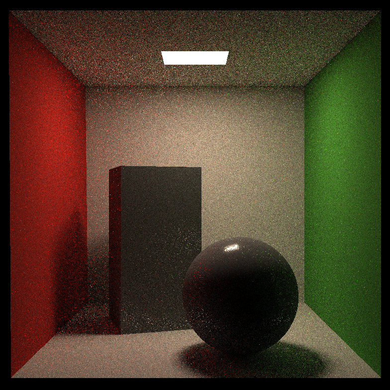
微表面模型
所有的 PBR 技术都基于微表面理论。这项理论认为,达到微观尺度之后任何表面都可以用被称为微表面 (Microfacets) 的细小镜面来进行描绘。在微观尺度下,没有任何表面是完全光滑的。然而由于这些微表面已经微小到无法逐像素的继续对其进行区分,因此我们只有假设一个粗糙度 (Roughness) 参数,然后用统计学的方法来概略的估算微表面的粗糙程度。
BRDF
性质
f ( i , o ) = F ( i , h ) G ( i , o , h ) D ( h ) 4 ( n , i ) ( n , o ) f(i,o)=\frac{F(i,h)G(i,o,h)D(h)}{4(n,i)(n,o)} f ( i , o ) = 4 ( n , i ) ( n , o ) F ( i , h ) G ( i , o , h ) D ( h )
F:菲涅尔方程,定义不同表面角下,表面所反射光线占比。
代码实现
这里参考 LearnOpenGL 给出的实现。
菲涅尔方程的近似
这里在 0.04 - ALBEDO (0.96) 间用金属度做插值,0.04 为基础反射率,0.96 接近于铝的反射率。
1 2 3 4 5 6 7 8 #define ALBEDO 0.96f float FresnelSchlick (const Vector3f& H, const Vector3f& V, const float & metalness) const float inter = 0.04f * (1 - metalness) + ALBEDO * metalness;float cosTheta = std::max (dotProduct (H, V), 0.f );return inter + (1.f - inter) * pow (1.f - cosTheta, 5.f );
法线分布模型
1 2 3 4 5 6 7 8 9 10 11 12 13 float DistributionGGX (Vector3f N, Vector3f H, float roughness) float a = roughness * roughness;float a2 = a * a;float NdotH = std::max (dotProduct (N, H), 0.f );float NdotH2 = NdotH * NdotH;float nom = a2;float denom = (NdotH2 * (a2 - 1.f ) + 1.f );return nom / std::max (denom, 1e-5f );
几何函数
1
2
3
4
5
6
7
8
9
10
11
12
13
14
15
16
17
18
float GeometrySchlickGGX (float NdotV, float roughness) float r = (roughness + 1.f );float k = (r * r) / 8.f ;float nom = NdotV;float denom = NdotV * (1.f - k) + k;return nom / std::max (denom, 1e-5f );float GeometrySmith (Vector3f N, Vector3f V, Vector3f L, float roughness) float NdotV = std::max (dotProduct (N, V), 0.f );float NdotL = std::max (dotProduct (N, L), 0.f );float ggx2 = GeometrySchlickGGX (NdotV, roughness);float ggx1 = GeometrySchlickGGX (NdotL, roughness);return ggx1 * ggx2;
BRDF
1 2 3 4 5 6 7 8 9 10 11 12 13 14 15 16 17 18 19 20 21 22 23 24 25 26 27 28 29 30 31 32 33 34 35 36 37 38 39 40 41 42 43 44 45 46 47 48 49 50 51 52 #define ALBEDO 0.96f Vector3f Material::eval (const Vector3f &wi, const Vector3f &wo, const Vector3f &N) {switch (m_type){case DIFFUSE:float cosalpha = dotProduct (N, wo);if (cosalpha > 0.f ) {return diffuse;else return Vector3f (0.f );break ;case Microfacet:float cosalpha = dotProduct (N, wo);if (cosalpha > 0.f ) {float roughness = 0.9f ;float metallic = 0.9f ;normalize (V + L);float F = Material::FresnelSchlick (H, V, metallic);float G = Material::GeometrySmith (N, V, L, roughness);float D = Material::DistributionGGX (N, H, roughness);float denominator = 4 * std::max (dotProduct (N, V), 0.f ) * max (dotProduct (N, L), 0.f );max (denominator, 1e-5f );Vector3f (1.f ) - kS;Vector3f (1.f - metallic);return kD * diffuse + specular;else return Vector3f (0.f );break ;
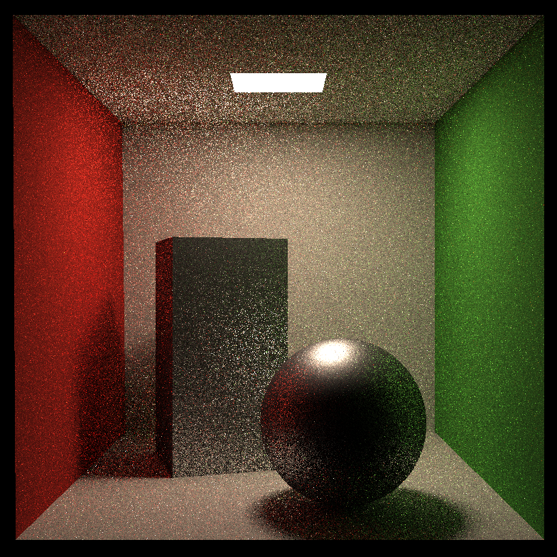
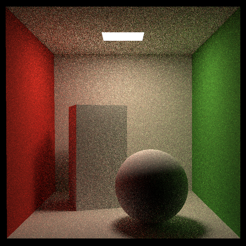
结果
相关链接
LearnOpenGL